13 Exercises IIIb

\[ \newcommand{\tr}{\mathrm{tr}} \newcommand{\rank}{\mathrm{rank}} \newcommand{\plim}{\operatornamewithlimits{plim}} \newcommand{\diag}{\mathrm{diag}} \newcommand{\bm}[1]{\boldsymbol{\mathbf{#1}}} \newcommand{\Var}{\mathrm{Var}} \newcommand{\Exp}{\mathrm{E}} \newcommand{\Cov}{\mathrm{Cov}} \newcommand\given[1][]{\:#1\vert\:} \newcommand{\irow}[1]{% \begin{pmatrix}#1\end{pmatrix} } \]

Required packages

pkgs <- c("sf", "mapview", "spdep", "spatialreg", "ggplot2", "tmap", "viridis", "viridisLite", 
          "plm", "lfe", "splm", "SDPDmod")
lapply(pkgs, require, character.only = TRUE)

Session info

sessionInfo()

R version 4.6.0 (2026-04-24 ucrt)
Platform: x86_64-w64-mingw32/x64
Running under: Windows 11 x64 (build 26200)

Matrix products: default
  LAPACK version 3.12.1

locale:
[1] LC_COLLATE=German_Germany.utf8  LC_CTYPE=German_Germany.utf8   
[3] LC_MONETARY=German_Germany.utf8 LC_NUMERIC=C                   
[5] LC_TIME=German_Germany.utf8    

time zone: Europe/Berlin
tzcode source: internal

attached base packages:
[1] stats     graphics  grDevices utils     datasets  methods  
[7] base     

other attached packages:
 [1] SDPDmod_0.0.7     splm_1.6-5        lfe_3.1.1        
 [4] plm_2.6-7         viridis_0.6.5     viridisLite_0.4.3
 [7] tmap_4.4          ggplot2_4.0.3     spatialreg_1.4-3 
[10] Matrix_1.7-5      spdep_1.4-2       spData_2.3.5     
[13] mapview_2.11.4    sf_1.1-1         

loaded via a namespace (and not attached):
  [1] Rdpack_2.6.6           DBI_1.3.0             
  [3] deldir_2.0-4           gridExtra_2.3         
  [5] tmaptools_3.3          s2_1.1.11             
  [7] logger_0.4.2           sandwich_3.1-1        
  [9] rlang_1.2.0            magrittr_2.0.5        
 [11] dreamerr_1.5.0         multcomp_1.4-30       
 [13] otel_0.2.0             e1071_1.7-17          
 [15] compiler_4.6.0         png_0.1-9             
 [17] vctrs_0.7.3            stringr_1.6.0         
 [19] pkgconfig_2.0.3        wk_0.9.5              
 [21] fastmap_1.2.0          backports_1.5.1       
 [23] lwgeom_0.2-16          leafem_0.2.5          
 [25] rmarkdown_2.31         spacesXYZ_1.6-0       
 [27] miscTools_0.6-30       xfun_0.57             
 [29] satellite_1.0.6        jsonlite_2.0.0        
 [31] stringmagic_1.2.0      collapse_2.1.7        
 [33] terra_1.9-27           parallel_4.6.0        
 [35] LearnBayes_2.15.2      R6_2.6.1              
 [37] stringi_1.8.7          RColorBrewer_1.1-3    
 [39] boot_1.3-32            numDeriv_2016.8-1.1   
 [41] lmtest_0.9-40          stars_0.7-2           
 [43] Rcpp_1.1.1-1.1         knitr_1.51            
 [45] zoo_1.8-15             base64enc_0.1-6       
 [47] splines_4.6.0          tidyselect_1.2.1      
 [49] rstudioapi_0.18.0      abind_1.4-8           
 [51] maptiles_0.11.0        maxLik_1.5-2.2        
 [53] codetools_0.2-20       lattice_0.22-9        
 [55] tibble_3.3.1           leafsync_0.1.0        
 [57] withr_3.0.2            S7_0.2.2              
 [59] coda_0.19-4.1          evaluate_1.0.5        
 [61] marginaleffects_0.32.0 survival_3.8-6        
 [63] fixest_0.14.1          units_1.0-1           
 [65] proxy_0.4-29           pillar_1.11.1         
 [67] KernSmooth_2.23-26     stats4_4.6.0          
 [69] generics_0.1.4         sp_2.2-1              
 [71] scales_1.4.0           xtable_1.8-8          
 [73] class_7.3-23           glue_1.8.1            
 [75] tools_4.6.0            leaflegend_1.2.8      
 [77] data.table_1.18.4      RSpectra_0.16-2       
 [79] dotCall64_1.2          mvtnorm_1.3-7         
 [81] XML_3.99-0.23          grid_4.6.0            
 [83] rbibutils_2.4.1        crosstalk_1.2.2       
 [85] bdsmatrix_1.3-7        colorspace_2.1-2      
 [87] nlme_3.1-169           cols4all_0.10         
 [89] raster_3.6-32          Formula_1.2-5         
 [91] cli_3.6.6              spam_2.11-4           
 [93] dplyr_1.2.1            gtable_0.3.6          
 [95] digest_0.6.39          classInt_0.4-11       
 [97] TH.data_1.1-5          htmlwidgets_1.6.4     
 [99] farver_2.1.2           htmltools_0.5.9       
[101] lifecycle_1.0.5        leaflet_2.2.3         
[103] microbenchmark_1.5.0   MASS_7.3-65

13.1 Inkar data: the effect of regional characteristics on life expectancy

Below, we read and transform some characteristics of the INKAR data on the level of German counties.

load("_data/inkar2.Rdata")

Variables are

Variable	Description
“Kennziffer”	ID
“Raumeinheit”	Name
“Aggregat”	Level
“year”	Year
“poluation_density”	Population Density
“median_income”	Median Household income (only for 2020)
“gdp_in1000EUR”	Gross Domestic Product in 1000 euros
“unemployment_rate”	Unemployment rate
“share_longterm_unemployed”	Share of longterm unemployed (among unemployed)
“share_working_indutry”	Share of employees in undistrial sector
“share_foreigners”	Share of foreign nationals
“share_college”	Share of school-finishers with college degree
“recreational_space”	Recreational space per inhabitant
“car_density”	Density of cars
“life_expectancy”	Life expectancy

13.2 County shapes

kreise.spdf <- st_read(dsn = "_data/vg5000_ebenen_1231",
                       layer = "VG5000_KRS")

Reading layer `VG5000_KRS' from data source 
  `C:\work\Lehre\Geodata_Spatial_Regression\_data\vg5000_ebenen_1231' 
  using driver `ESRI Shapefile'
Simple feature collection with 400 features and 24 fields
Geometry type: MULTIPOLYGON
Dimension:     XY
Bounding box:  xmin: 280353.1 ymin: 5235878 xmax: 921261.6 ymax: 6101302
Projected CRS: ETRS89 / UTM zone 32N

1) Please map the life expectancy across Germany

Merge data with the shape file (as with conventional data)
Create a map of life-expectancy

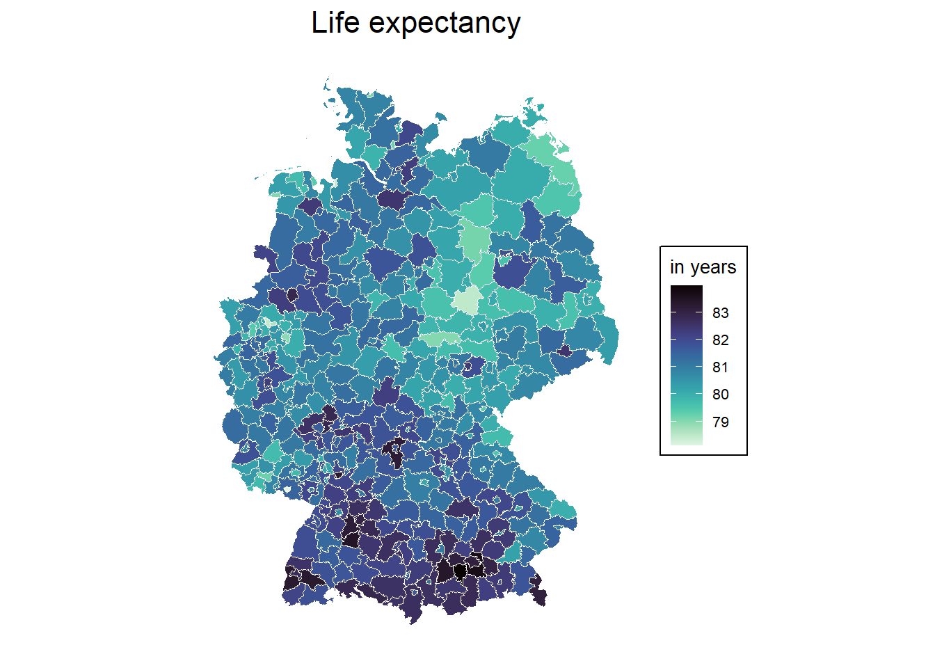
2) We want to know what the predicts the variation in life expectancy. Chose some variables that could predict life expectancy. See for instance the following paper.

3) Obviously, as good geospatial scholars, we might assume that it is not only the focal characteristics that matter, but maybe also the characteristics of surrounding counties. Please create a neighbours object such as the 10 nearest neighbours.

4) Please estimate a cross-sectional spatial model for the year 2020 that predicts life expectancy (as the depend variable) with the covariates that you have choosen above. Afterwards, please calculate the summary impacts using `impacts()`.

5) Calculate the spatial lagged variables for the independent variables that you have included in the earlier model. You can use `create_WX()`, but note that it needs a non-spatial df as input for the original variables.

6) Bonus task: Can you run a spatial machine learning model?

For instance, you could use a random forest algorithm (e.g. randomForest()) and include the original variables but also the spatial lags of these variables. You could even go further and use higher order neighbours (e.g. nblag(queens.nb, maxlag = 3)) to check the importance of direct neighbours and the neighbours neighbours and so on …

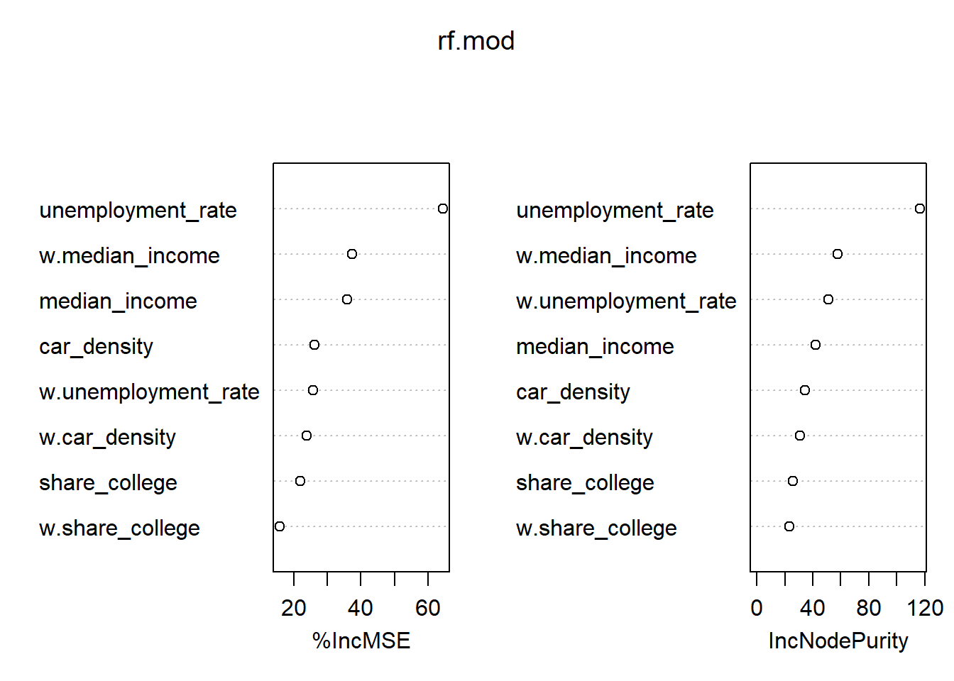
13.3 Bonus task: Estimate an FE model with SLX specification

Loop over years to generate WX
Estimate a twoways FE SLX panel model
Estimate a twoways FE SAR panel model (use spml())
Estimate the summary impacts.

Note that for some reason, the new version of impacts() in spatialreg looks for the attribute “have_factor_preds”, Which is not present in the splm object. So have to manually assign it via attr(sar.fe, "have_factor_preds") <- FALSE.

::: {.content-hidden unless-format="html"} $$ \newcommand{\tr}{\mathrm{tr}} \newcommand{\rank}{\mathrm{rank}} \newcommand{\plim}{\operatornamewithlimits{plim}} \newcommand{\diag}{\mathrm{diag}} \newcommand{\bm}[1]{\boldsymbol{\mathbf{#1}}} \newcommand{\Var}{\mathrm{Var}} \newcommand{\Exp}{\mathrm{E}} \newcommand{\Cov}{\mathrm{Cov}} \newcommand\given[1][]{\:#1\vert\:} \newcommand{\irow}[1]{% \begin{pmatrix}#1\end{pmatrix} } $$ ::: # Exercises IIIb ### Required packages {.unnumbered} ```{r, message = FALSE, warning = FALSE, results = 'hide'} pkgs <- c("sf", "mapview", "spdep", "spatialreg", "ggplot2", "tmap", "viridis", "viridisLite", "plm", "lfe", "splm", "SDPDmod") lapply(pkgs, require, character.only = TRUE) ``` ### Session info {.unnumbered} ```{r} sessionInfo() ``` ## Inkar data: the effect of regional characteristics on life expectancy Below, we read and transform some characteristics of the [INKAR data](https://www.inkar.de/) on the level of German counties.                                                                             ```{r} load("_data/inkar2.Rdata") ``` Variables are | Variable | Description | | ------------ | ------------ | | "Kennziffer" | ID | | "Raumeinheit" | Name | | "Aggregat" | Level | | "year" | Year | | "poluation_density" | Population Density | | "median_income" | Median Household income (only for 2020) | | "gdp_in1000EUR" | Gross Domestic Product in 1000 euros | | "unemployment_rate" | Unemployment rate | | "share_longterm_unemployed" | Share of longterm unemployed (among unemployed) | | "share_working_indutry" | Share of employees in undistrial sector | | "share_foreigners" | Share of foreign nationals | | "share_college" | Share of school-finishers with college degree | | "recreational_space" | Recreational space per inhabitant | | "car_density" | Density of cars | | "life_expectancy" | Life expectancy | ## County shapes ```{r} kreise.spdf <- st_read(dsn = "_data/vg5000_ebenen_1231", layer = "VG5000_KRS") ``` ### 1) Please map the life expectancy across Germany {.unnumbered} a) Merge data with the shape file (as with conventional data) b) Create a map of life-expectancy ### 2) We want to know what the predicts the variation in life expectancy. Chose some variables that could predict life expectancy. See for instance the [following paper](https://doi.org/10.1073/pnas.2003719117). {.unnumbered} ### 3) Obviously, as good geospatial scholars, we might assume that it is not only the focal characteristics that matter, but maybe also the characteristics of surrounding counties. Please create a neighbours object such as the 10 nearest neighbours. {.unnumbered} ### 4) Please estimate a cross-sectional spatial model for the year 2020 that predicts life expectancy (as the depend variable) with the covariates that you have choosen above. Afterwards, please calculate the summary impacts using `impacts()`. {.unnumbered} ### 5) Calculate the spatial lagged variables for the independent variables that you have included in the earlier model. You can use `create_WX()`, but note that it needs a non-spatial df as input for the original variables. {.unnumbered} ### 6) Bonus task: Can you run a spatial machine learning model? {.unnumbered} For instance, you could use a random forest algorithm (e.g. `randomForest()`) and include the original variables but also the spatial lags of these variables. You could even go further and use higher order neighbours (e.g. `nblag(queens.nb, maxlag = 3)`) to check the importance of direct neighbours and the neighbours neighbours and so on ... ## Bonus task: Estimate an FE model with SLX specification a) Loop over years to generate WX b) Estimate a twoways FE SLX panel model c) Estimate a twoways FE SAR panel model (use `spml()`) d) Estimate the summary impacts. Note that for some reason, the new version of `impacts()` in `spatialreg` looks for the attribute "have_factor_preds", Which is not present in the `splm` object. So have to manually assign it via `attr(sar.fe, "have_factor_preds") <- FALSE`.