2 Data Manipulation & Visualization
\[ \newcommand{\tr}{\mathrm{tr}} \newcommand{\rank}{\mathrm{rank}} \newcommand{\plim}{\operatornamewithlimits{plim}} \newcommand{\diag}{\mathrm{diag}} \newcommand{\bm}[1]{\boldsymbol{\mathbf{#1}}} \newcommand{\Var}{\mathrm{Var}} \newcommand{\Exp}{\mathrm{E}} \newcommand{\Cov}{\mathrm{Cov}} \newcommand\given[1][]{\:#1\vert\:} \newcommand{\irow}[1]{% \begin{pmatrix}#1\end{pmatrix} } \]
Required packages
For mapping
Session info
R version 4.6.0 (2026-04-24 ucrt)
Platform: x86_64-w64-mingw32/x64
Running under: Windows 11 x64 (build 26200)
Matrix products: default
LAPACK version 3.12.1
locale:
[1] LC_COLLATE=German_Germany.utf8 LC_CTYPE=German_Germany.utf8
[3] LC_MONETARY=German_Germany.utf8 LC_NUMERIC=C
[5] LC_TIME=German_Germany.utf8
time zone: Europe/Berlin
tzcode source: internal
attached base packages:
[1] stats graphics grDevices utils datasets methods
[7] base
other attached packages:
[1] gridExtra_2.3 cowplot_1.2.0 rmapshaper_0.6.1
[4] ggthemes_5.2.0 ggplot2_4.0.3 viridis_0.6.5
[7] viridisLite_0.4.3 tmaptools_3.3 tmap_4.4
[10] xml2_1.5.2 downlit_0.4.5 texreg_1.39.5
[13] tidyr_1.3.2 OpenStreetMap_0.4.1 osmdata_0.3.0
[16] areal_0.1.8 dplyr_1.2.1 rnaturalearth_1.2.0
[19] nngeo_0.4.8 mapview_2.11.4 gstat_2.1-6
[22] sf_1.1-1
loaded via a namespace (and not attached):
[1] tidyselect_1.2.1 farver_2.1.2 S7_0.2.2
[4] fastmap_1.2.0 leaflegend_1.2.8 leaflet_2.2.3
[7] XML_3.99-0.23 digest_0.6.39 lifecycle_1.0.5
[10] terra_1.9-27 magrittr_2.0.5 compiler_4.6.0
[13] rlang_1.2.0 tools_4.6.0 data.table_1.18.4
[16] knitr_1.51 FNN_1.1.4.1 htmlwidgets_1.6.4
[19] curl_7.1.0 sp_2.2-1 classInt_0.4-11
[22] RColorBrewer_1.1-3 abind_1.4-8 KernSmooth_2.23-26
[25] withr_3.0.2 purrr_1.2.2 leafsync_0.1.0
[28] grid_4.6.0 stats4_4.6.0 xts_0.14.2
[31] cols4all_0.10 e1071_1.7-17 leafem_0.2.5
[34] colorspace_2.1-2 spacesXYZ_1.6-0 scales_1.4.0
[37] cli_3.6.6 rmarkdown_2.31 intervals_0.15.5
[40] generics_0.1.4 otel_0.2.0 rstudioapi_0.18.0
[43] httr_1.4.8 DBI_1.3.0 cachem_1.1.0
[46] proxy_0.4-29 stringr_1.6.0 stars_0.7-2
[49] parallel_4.6.0 s2_1.1.11 base64enc_0.1-6
[52] vctrs_0.7.3 V8_8.2.0 jsonlite_2.0.0
[55] crosstalk_1.2.2 units_1.0-1 maptiles_0.11.0
[58] glue_1.8.1 lwgeom_0.2-16 codetools_0.2-20
[61] stringi_1.8.7 rJava_1.0-18 gtable_0.3.6
[64] raster_3.6-32 tibble_3.3.1 logger_0.4.2
[67] pillar_1.11.1 htmltools_0.5.9 satellite_1.0.6
[70] R6_2.6.1 wk_0.9.5 microbenchmark_1.5.0
[73] evaluate_1.0.5 lattice_0.22-9 png_0.1-9
[76] memoise_2.0.1 class_7.3-23 Rcpp_1.1.1-1.1
[79] spacetime_1.3-3 xfun_0.57 zoo_1.8-15
[82] pkgconfig_2.0.3 Reload data from pervious session
2.1 Manipulation and linkage
Having data with geo-spatial information allows to perform a variety of methods to manipulate and link different data sources. Commonly used methods include 1) subsetting, 2) point-in-polygon operations, 3) distance measures, 4) intersections or buffer methods.
The online Vignettes of the sf package provide a comprehensive overview of the multiple ways of spatial manipulations.
Check if data is on common projection
st_crs(msoa.spdf) == st_crs(pol.spdf)[1] FALSEst_crs(msoa.spdf) == st_crs(pubs.spdf)[1] FALSEst_crs(msoa.spdf) == st_crs(ulez.spdf)[1] FALSEThe spatial data files are on different projections. Before we can do any spatial operations with them, we have to transform them into a common projection.
# MSOA in different crs --> transform
pol.spdf <- st_transform(pol.spdf, crs = st_crs(msoa.spdf))
pubs.spdf <- st_transform(pubs.spdf, crs = st_crs(msoa.spdf))
ulez.spdf <- st_transform(ulez.spdf, crs = st_crs(msoa.spdf))
# Check if all geometries are valid, and make valid if needed
msoa.spdf <- st_make_valid(msoa.spdf)The st_make_valid() function can help if the spatial geometries have some problems such as holes or points that don’t match exactly.
2.1.1 Subsetting
We can subset spatial data in a similar way as we subset conventional data.frames or matrices. For instance, below we simply reduce the pollution grid across the UK to observations in London only.
# Subset to pollution estimates in London
pol_sub.spdf <- pol.spdf[msoa.spdf, ] # or:
pol_sub.spdf <- st_filter(pol.spdf, msoa.spdf)
mapview(pol_sub.spdf)Or we can reverse the above and exclude all intersecting units by specifying st_disjoint as alternative spatial operation using the op = option (note the empty space for column selection). st_filter() with the .predicate option does the same job. See the sf Vignette for more operations.
# Subset pubs to pubs not in the ulez area
sub2.spdf <- pubs.spdf[ulez.spdf, , op = st_disjoint] # or:
sub2.spdf <- st_filter(pubs.spdf, ulez.spdf, .predicate = st_disjoint)
mapview(sub2.spdf)We can easily create indicators of whether an MSOA is within ulez or not.
2.1.2 Point in polygon
We are interested in the number of pubs in each MSOA. So, we count the number of points in each polygon.
[1] 16012.1.3 Distance measures
We might be interested in the distance to the nearest pub. Here, we use the package nngeo to find k nearest neighbours with the respective distance.
# Use geometric centroid of each MSOA
cent.sp <- st_centroid(msoa.spdf[, "MSOA11CD"])Warning: st_centroid assumes attributes are constant over
geometries# Get K nearest neighbour with distance
knb.dist <- st_nn(cent.sp,
pubs.spdf,
k = 1, # number of nearest neighbours
returnDist = TRUE, # we also want the distance
progress = FALSE)projected points Min. 1st Qu. Median Mean 3rd Qu. Max.
9.079 305.149 565.018 701.961 948.047 3735.478 2.1.4 Intersections + Buffers
We may also want the average pollution within 1 km radius around each MSOA centroid. Note that it is usually better to use a ego-centric method where you calculate the average within a distance rather than using the characteristic of the intersecting cells only (Lee et al. 2008; Mohai and Saha 2007).
To do this, we first create a 1 km buffer around each centroid using st_buffer(). Obviously, you could also use the existing polygons (e.g. each LSOA shape) rather than such a buffer around the mid/point. We then use area-weighted interpolation from the areal package to estimate average pollution values within each buffer. This approach accounts for the proportion of each pollution grid cell that overlaps with the buffer area and provides a more streamlined alternative to manually calculating intersections and weighted averages.
In the commented section below, you also see an older version that uses st_intersetion() to calculate the overlap manually.
# Create buffer (1km radius)
cent.buf <- st_buffer(cent.sp,
dist = 1000) # dist in meters
mapview(cent.buf)### New version (using areal package)
# We use area-weighted interpolation from the areal package
int.spdf <- aw_interpolate(
cent.buf, # interpolate to
tid = "MSOA11CD", # id of target
source = pol.spdf, # the source to be interpolated from
sid = "ukgridcode", # source id
weight = "sum", # function for interpolation
output = "sf", # output object
intensive = "no22011" # variables to be interpolated
)
# # ### Old version ("by hand")
# # Add area of each buffer (in this constant)
# cent.buf$area <- as.numeric(st_area(cent.buf))
#
# # Calculate intersection of pollution grid and buffer
# int.df <- st_intersection(cent.buf, pol.spdf)
# int.df$int_area <- as.numeric(st_area(int.df)) # area of intersection
#
# # And we use the percent overlap areas as the weights to calculate a weighted mean.
#
# # Area of intersection as share of buffer
# int.df$area_per <- int.df$int_area / int.df$area
#
# # Aggregate as weighted mean
# int.df <- st_drop_geometry(int.df)
# int.df$no2_weighted <- int.df$no22011 * int.df$area_per
# int.df <- aggregate(list(no2 = int.df[, "no2_weighted"]),
# by = list(MSOA11CD = int.df$MSOA11CD),
# sum)And we merge that back to the LSOA data.
Note: for buffer related methods, it often makes sense to use population weighted centroids instead of geographic centroids (see here for MSOA population weighted centroids). However, often this information is not available.
2.1.5 and more
There are more spatial operation possible using sf. Have a look at the sf Cheatsheet.
2.1.6 Air pollution and ethnic minorities
With a few lines of code, we have compiled an original dataset containing demographic information, air pollution, and some infrastructural information.
Let’s see what we can do with it.
# Define ethnic group shares
msoa.spdf$per_mixed <- msoa.spdf$KS201EW_200 / msoa.spdf$KS201EW0001 * 100
msoa.spdf$per_asian <- msoa.spdf$KS201EW_300 / msoa.spdf$KS201EW0001 * 100
msoa.spdf$per_black <- msoa.spdf$KS201EW_400 / msoa.spdf$KS201EW0001 * 100
msoa.spdf$per_other <- msoa.spdf$KS201EW_500 / msoa.spdf$KS201EW0001 * 100
# Define tenure
msoa.spdf$per_owner <- msoa.spdf$KS402EW_100 / msoa.spdf$KS402EW0001 * 100
msoa.spdf$per_social <- msoa.spdf$KS402EW_200 / msoa.spdf$KS402EW0001 * 100
# Non British passport
msoa.spdf$per_nonUK <- (msoa.spdf$KS205EW0001 - msoa.spdf$KS205EW0003)/ msoa.spdf$KS205EW0001 * 100
msoa.spdf$per_nonEU <- (msoa.spdf$KS205EW0001 - msoa.spdf$KS205EW0003 -
msoa.spdf$KS205EW0004 - msoa.spdf$KS205EW0005 -
msoa.spdf$KS205EW0006)/ msoa.spdf$KS205EW0001 * 100
msoa.spdf$per_nonUK_EU <- (msoa.spdf$KS205EW0005 + msoa.spdf$KS205EW0006)/ msoa.spdf$KS205EW0001 * 100
# Run regression
mod1.lm <- lm(no2 ~ per_mixed + per_asian + per_black + per_other +
per_owner + per_social + pubs_count + POPDEN + ulez,
data = msoa.spdf)
# summary
screenreg(list(mod1.lm), digits = 3)
========================
Model 1
------------------------
(Intercept) 37.112 ***
(1.308)
per_mixed -0.090
(0.099)
per_asian 0.018 *
(0.007)
per_black -0.085 ***
(0.016)
per_other 0.462 ***
(0.047)
per_owner -0.207 ***
(0.013)
per_social -0.058 ***
(0.013)
pubs_count 0.218 ***
(0.040)
POPDEN 0.037 ***
(0.003)
ulez 9.556 ***
(0.686)
------------------------
R^2 0.774
Adj. R^2 0.772
Num. obs. 983
========================
*** p < 0.001; ** p < 0.01; * p < 0.05For some examples later, we also add data on house prices. We use the median house prices in 2017 from the London Datastore.
Year ending Dec 2011 Year ending Jun 2011 Year ending Mar 2011
983 983 983
Year ending Sep 2011
983 # Aggregate across 2011 values
hp.df$med_house_price <- as.numeric(hp.df$Value)
hp.df <- aggregate(hp.df[, "med_house_price", drop = FALSE],
by = list(MSOA11CD = hp.df$Code),
FUN = function(x) mean(x, na.rm = TRUE))
# Merge spdf and housing prices
msoa.spdf <- merge(msoa.spdf, hp.df,
by = "MSOA11CD",
all.x = TRUE, all.y = FALSE)
hist(log(msoa.spdf$med_house_price))
2.1.7 Save spatial data
# Save
save(msoa.spdf, file = "_data/msoa2_spatial.RData")2.2 Visualization
A large advantage of spatial data is that different data sources can be connected and combined. Another nice advantage is: you can create very nice maps. And it’s quite easy to do! Stefan Jünger & Anne-Kathrin Stroppe provide more comprehensive materials on mapping in their GESIS workshop on geospatial techniques in R.
Many packages and functions can be used to plot maps of spatial data. For instance, ggplot as a function to plot spatial data using geom_sf(). I am personally a fan of tmap, which makes many steps easier (but sometimes is less flexible).
A great tool for choosing coulour is for instance Colorbrewer. viridis provides another great resource to chose colours.
2.2.1 ggplot
Many of you will be familiar with ggplot. Obviously, you can also create very nice maps with ggplot and the geom_sf() layer. Particularly for continuous scales which you don’t want to cut into bins, ggplot is probably the best choice. The options coord_sf(datum = NA) and theme_map() help to improve the layout (e.g. omitting the scales and the ticks).
gp <- ggplot(msoa.spdf)+
geom_sf(aes(fill = no2))+
scale_fill_viridis_c(option = "B")+
coord_sf(datum = NA)+
theme_map()+
theme(legend.position = c(.9, .6))
gp
As always with ggplot, we can add different layers of data on top of each other. Below, we combine different layers of geom_sf().
# Get some larger scale boundaries
borough.spdf <- st_read(
dsn = paste0("_data", "/statistical-gis-boundaries-london/ESRI"),
layer = "London_Borough_Excluding_MHW" # Note: no file ending
)Reading layer `London_Borough_Excluding_MHW' from data source
`C:\work\Lehre\Geodata_Spatial_Regression\_data\statistical-gis-boundaries-london\ESRI'
using driver `ESRI Shapefile'
Simple feature collection with 33 features and 7 fields
Geometry type: MULTIPOLYGON
Dimension: XY
Bounding box: xmin: 503568.2 ymin: 155850.8 xmax: 561957.5 ymax: 200933.9
Projected CRS: OSGB36 / British National Grid# transform to only inner lines
borough_inner <- ms_innerlines(borough.spdf)
# Plot with inner lines
gp <- ggplot(msoa.spdf) +
geom_sf(aes(fill = no2), color = NA) +
scale_fill_viridis_c(option = "A") +
geom_sf(data = borough_inner, color = "gray92") +
geom_sf(
data = ulez.spdf,
color = "red",
fill = NA,
linewidth = 1.5
) +
coord_sf(datum = NA) +
theme_map() +
labs(fill = "NO2 in mg/m3", title = "Air pollution") +
theme(legend.position = c(.7, .3),
plot.title = element_text(hjust = 0.5, size = 18),
legend.background = element_rect(fill = "white", color = NA))
gp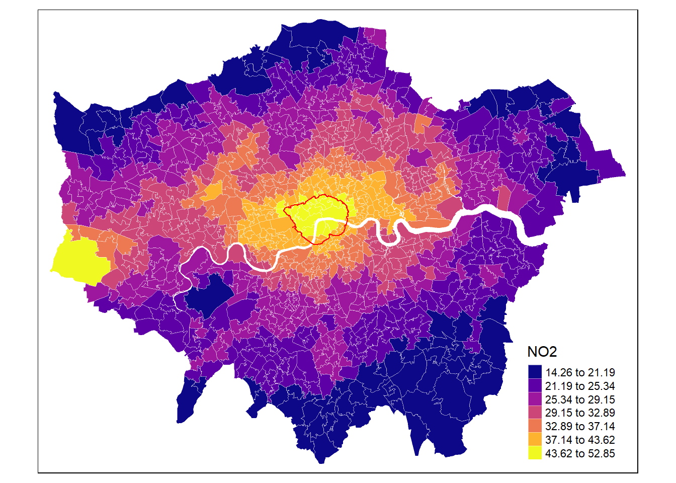
And we can combine single maps, e.g. with the gridExtra package and the grid.arrange() function. We use exactly the same function, and only change the colouring option in scale_fill_viridis_c() which is the viridis colour option for continuous scales.
# Plot with inner lines
gp2 <- ggplot(msoa.spdf) +
geom_sf(aes(fill = med_house_price/1000), color = NA) +
scale_fill_viridis_c(option = "D") +
geom_sf(data = borough_inner, color = "gray92") +
geom_sf(
data = ulez.spdf,
color = "red",
fill = NA,
linewidth = 1.5
) +
coord_sf(datum = NA) +
theme_map() +
labs(fill = "Median/1000", title = "House price") +
theme(legend.position = c(.7, .3),
plot.title = element_text(hjust = 0.5, size = 18),
legend.background = element_rect(fill = "white", color = NA))
gpc <- grid.arrange(gp, gp2, ncol = 2, nrow = 1)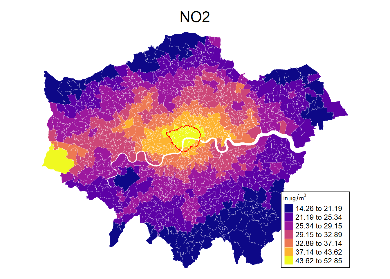
plot(gpc)And we can use the standard functions to export a png is good resolution.
2.2.2 Tmaps
Another nice package for data visualisation is tmp. It’s particularly nice, if you want to cut the colour into different brackets / bins. The tm_scale_intervals() function provides very helpful algorithms to cut the variable range into different bins for colouring.
For instance, lets plot the NO2 estimates using tmap + tm_polygon() and the fisher algorithm for the colour intervals.
# Define colours
cols <- viridis(n = 7, direction = 1, option = "C")
mp1 <- tm_shape(msoa.spdf) +
tm_polygons(
fill = "no2", # variable for fill colouring
fill_alpha = 1, # transparency
fill.scale = tm_scale_intervals(
style = "fisher", # algorithm to def cut points
n = 7, # Number of requested cut points
values = cols # colouring
),
fill.legend = tm_legend(
title = "NO2",
hist = FALSE
)
) +
tm_borders(
col = "white",
lwd = 0.5,
fill_alpha = 0.5
)
mp1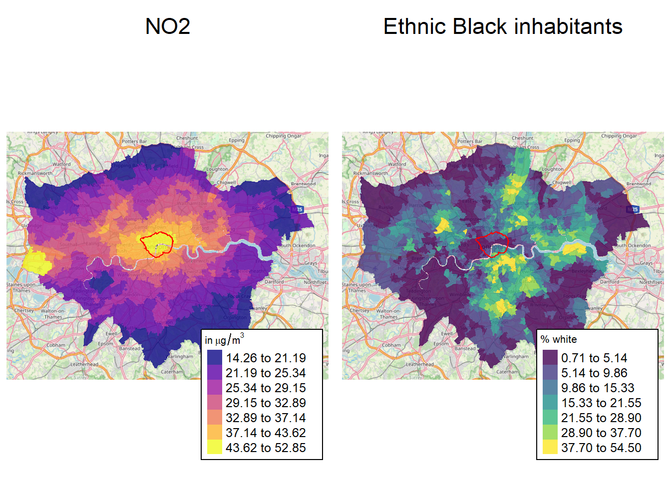
Tmap allows to easily combine different objects by defining a new object via tm_shape().
# Define colours
cols <- viridis(n = 7, direction = 1, option = "C")
mp1 <- tm_shape(msoa.spdf) +
tm_polygons(
fill = "no2",
fill_alpha = 1,
fill.scale = tm_scale_intervals(
style = "fisher",
n = 7,
values = cols
),
fill.legend = tm_legend(
title = "NO2",
hist = FALSE
)
) +
tm_borders(
col = "white",
lwd = 0.5,
fill_alpha = 0.5
) +
tm_shape(ulez.spdf) +
tm_borders(
col = "red",
lwd = 1,
fill_alpha = 1
)
mp1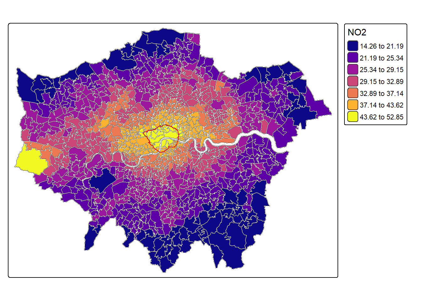
And it is easy to change the layout.
# Define colours
cols <- viridis(n = 7, direction = 1, option = "C")
mp1 <- tm_shape(msoa.spdf) +
tm_polygons(
fill = "no2",
fill_alpha = 1,
fill.scale = tm_scale_intervals(
style = "fisher",
n = 7,
values = cols
),
fill.legend = tm_legend(
title = expression('in'~mu*'g'/m^{3}),
hist = FALSE
)
) +
tm_borders(
col = "white",
lwd = 0.5,
fill_alpha = 0.5
) +
tm_shape(ulez.spdf) +
tm_borders(
col = "red",
lwd = 1,
fill_alpha = 1
) +
tm_layout(
frame = FALSE,
legend.frame = TRUE,
legend.bg.color = "white",
legend.position = c("right", "bottom"),
legend.outside = FALSE,
legend.title.size = 0.8,
legend.text.size = 0.8
) +
tm_title_out(
text = "NO2",
position = tm_pos_out("center", "top", # top cell
pos.h = "center"), # position in cell
size = 1.6
)
mp1
We can also add some map information from OSM. However, it’s sometimes a bit tricky with the projection. That’s why we switch into the OSM projection here. Note that this osm query is build on retiring packages.
# Save old projection
crs_orig <- st_crs(msoa.spdf)
# Change projection
ulez.spdf <- st_transform(ulez.spdf, 4326)
msoa.spdf <- st_transform(msoa.spdf, 4326)
# Get OSM data for background
osm_tmp <- read_osm(st_bbox(msoa.spdf), ext = 1.1, type = "osm-german")
# Define colours
cols <- viridis(n = 7, direction = 1, option = "C")
mp1 <- tm_shape(osm_tmp) +
tm_rgb() +
tm_shape(msoa.spdf) +
tm_polygons(
fill = "no2",
fill_alpha = 0.8,
fill.scale = tm_scale_intervals(
style = "fisher",
n = 7,
values = cols
),
fill.legend = tm_legend(
title = expression('in'~mu*'g'/m^{3}),
hist = FALSE
)
) +
tm_shape(ulez.spdf) +
tm_borders(
col = "red",
lwd = 1,
fill_alpha = 1
) +
tm_layout(
frame = FALSE,
legend.frame = TRUE,
legend.bg.color = "white",
legend.position = c("right", "bottom"),
legend.outside = FALSE,
legend.title.size = 0.8,
legend.text.size = 0.8
) +
tm_title_out(
text = "NO2",
position = tm_pos_out("center", "top", pos.h = "center"),
size = 1.6
)
mp1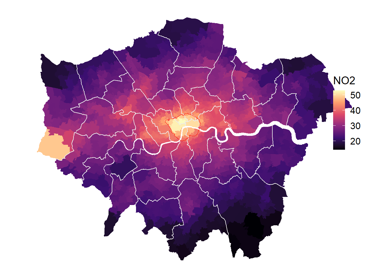
Tmap also makes it easy to combine single maps
# Define colours
cols1 <- viridis(n = 7, direction = 1, option = "C")
# Define colours
cols2 <- viridis(n = 7, direction = 1, option = "D")
# First map: NO2
mp1 <- tm_shape(osm_tmp) +
tm_rgb() +
tm_shape(msoa.spdf) +
tm_polygons(
fill = "no2",
fill_alpha = 0.8,
fill.scale = tm_scale_intervals(
style = "fisher",
n = 7,
values = cols1
),
fill.legend = tm_legend(
title = expression('in'~mu*'g'/m^{3}),
hist = FALSE
)
) +
tm_shape(ulez.spdf) +
tm_borders(
col = "red",
lwd = 1,
fill_alpha = 1
) +
tm_layout(
frame = FALSE,
legend.frame = TRUE,
legend.bg.color = "white",
legend.position = c("right", "bottom"),
legend.outside = FALSE,
legend.title.size = 0.8,
legend.text.size = 0.8
) +
tm_title_out(
text = "NO2",
position = tm_pos_out("center", "top", pos.h = "center"),
size = 1.4
)
# Second map: % Black
mp2 <- tm_shape(osm_tmp) +
tm_rgb() +
tm_shape(msoa.spdf) +
tm_polygons(
fill = "per_black",
fill_alpha = 0.8,
fill.scale = tm_scale_intervals(
style = "fisher",
n = 7,
values = cols2
),
fill.legend = tm_legend(
title = "% black",
hist = FALSE
)
) +
tm_shape(ulez.spdf) +
tm_borders(
col = "red",
lwd = 1,
fill_alpha = 1
) +
tm_layout(
frame = FALSE,
legend.frame = TRUE,
legend.bg.color = "white",
legend.position = c("right", "bottom"),
legend.outside = FALSE,
legend.title.size = 0.8,
legend.text.size = 0.8
) +
tm_title_out(
text = "Ethnic Black inhabitants",
position = tm_pos_out("center", "top", pos.h = "center"),
size = 1.4
)
# Arrange side by side
tmap_arrange(mp1, mp2, ncol = 2, nrow = 1)
And you can easily export those to png or pdf
2.3 Exercises
- What is the difference between a spatial “sf” object and a conventional “data.frame”? What’s the purpose of the function
st_drop_geometry()?
It’s the same. A spatial “sf” object just has an additional column containing the spatial coordinates.
- Using msoa.spdf, please create a spatial data frame that contains only the MSOA areas that are within the ulez zone.
sub4.spdf <- msoa.spdf[ulez.spdf, ]- Please create a map for London (or only the msoa-ulez subset) which shows the share of Asian residents (or any other ethnic group).
gp <- ggplot(msoa.spdf)+
geom_sf(aes(fill = per_asian))+
scale_fill_viridis_c(option = "E")+
coord_sf(datum = NA)+
theme_map()+
theme(legend.position = c(.9, .6))
gp
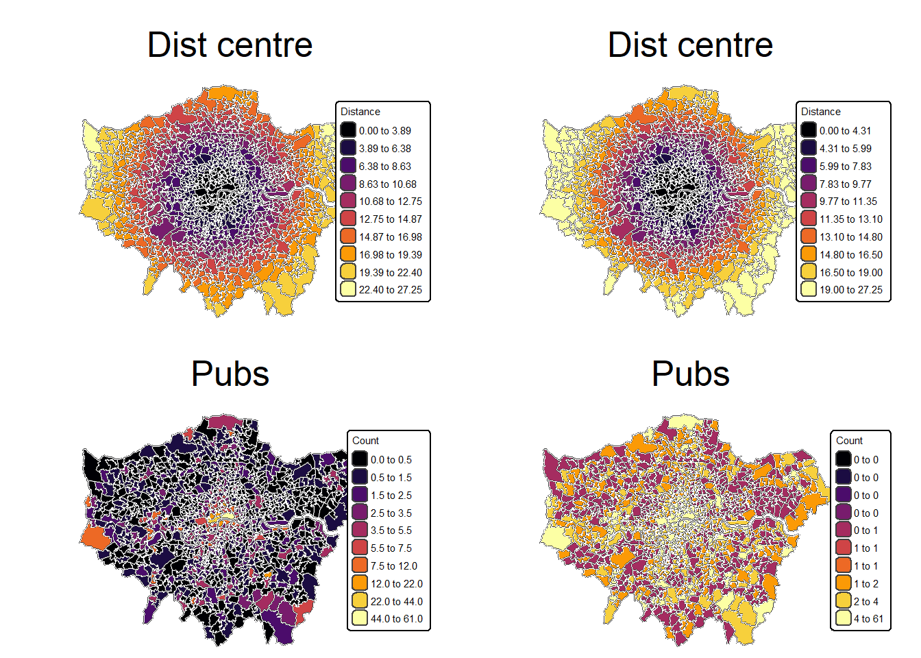
- Please calculate the distance of each MSOA to the London city centre
- use google maps to get lon and lat,
- use
st_as_sf()to create the spatial point - use
st_distance()to calculate the distance
### Distance to city center
# Define centre
centre <- st_as_sf(data.frame(lon = -0.128120855701165,
lat = 51.50725909644806),
coords = c("lon", "lat"),
crs = 4326)
# Reproject
centre <- st_transform(centre, crs = st_crs(msoa.spdf))
# Calculate distance
msoa.spdf$dist_centre <- as.numeric(st_distance(msoa.spdf, centre)) / 1000
# hist(msoa.spdf$dist_centre)- Can you create a plot with the distance to the city centre and pub counts next to each other?
# Define colours
cols <- viridis(n = 10, direction = 1, option = "B")
cols2 <- viridis(n = 10, direction = 1, option = "E")
library(tmap)
# Map 1: Distance - Fisher
mp1 <- tm_shape(msoa.spdf) +
tm_polygons(
fill = "dist_centre",
fill_alpha = 1,
fill.scale = tm_scale_intervals(
style = "fisher",
n = 10,
values = cols
),
fill.legend = tm_legend(
title = "Distance",
hist = FALSE
)
) +
tm_borders(col = "white", lwd = 0.5, fill_alpha = 0.5) +
tm_layout(
frame = FALSE,
legend.frame = TRUE,
legend.bg.color = "white",
legend.position = c("right", "bottom"),
legend.outside = FALSE,
legend.title.size = 0.8,
legend.text.size = 0.8
) +
tm_title_out(
text = "Dist centre",
position = tm_pos_out("center", "top", pos.h = "center"),
size = 1.6
)
# Map 2: Distance - Quantile
mp2 <- tm_shape(msoa.spdf) +
tm_polygons(
fill = "dist_centre",
fill_alpha = 1,
fill.scale = tm_scale_intervals(
style = "quantile",
n = 10,
values = cols
),
fill.legend = tm_legend(
title = "Distance",
hist = FALSE
)
) +
tm_borders(col = "white", lwd = 0.5, fill_alpha = 0.5) +
tm_layout(
frame = FALSE,
legend.frame = TRUE,
legend.bg.color = "white",
legend.position = c("right", "bottom"),
legend.outside = FALSE,
legend.title.size = 0.8,
legend.text.size = 0.8
) +
tm_title_out(
text = "Dist centre",
position = tm_pos_out("center", "top", pos.h = "center"),
size = 1.6
)
# Map 3: Pubs - Fisher
mp3 <- tm_shape(msoa.spdf) +
tm_polygons(
fill = "pubs_count",
fill_alpha = 1,
fill.scale = tm_scale_intervals(
style = "fisher",
n = 10,
values = cols
),
fill.legend = tm_legend(
title = "Count",
hist = FALSE
)
) +
tm_borders(col = "white", lwd = 0.5, fill_alpha = 0.5) +
tm_layout(
frame = FALSE,
legend.frame = TRUE,
legend.bg.color = "white",
legend.position = c("right", "bottom"),
legend.outside = FALSE,
legend.title.size = 0.8,
legend.text.size = 0.8
) +
tm_title_out(
text = "Pubs",
position = tm_pos_out("center", "top", pos.h = "center"),
size = 1.6
)
# Map 4: Pubs - Quantile
mp4 <- tm_shape(msoa.spdf) +
tm_polygons(
fill = "pubs_count",
fill_alpha = 1,
fill.scale = tm_scale_intervals(
style = "quantile",
n = 10,
values = cols
),
fill.legend = tm_legend(
title = "Count",
hist = FALSE
)
) +
tm_borders(col = "white", lwd = 0.5, fill_alpha = 0.5) +
tm_layout(
frame = FALSE,
legend.frame = TRUE,
legend.bg.color = "white",
legend.position = c("right", "bottom"),
legend.outside = FALSE,
legend.title.size = 0.8,
legend.text.size = 0.8
) +
tm_title_out(
text = "Pubs",
position = tm_pos_out("center", "top", pos.h = "center"),
size = 1.6
)
tmap_arrange(mp1, mp2, mp3, mp4, ncol = 2, nrow = 2)[plot mode] fit legend/component: Some legend items or map
compoments do not fit well, and are therefore rescaled.
ℹ Set the tmap option `component.autoscale = FALSE` to disable
rescaling.
[plot mode] fit legend/component: Some legend items or map
compoments do not fit well, and are therefore rescaled.
ℹ Set the tmap option `component.autoscale = FALSE` to disable
rescaling.
[plot mode] fit legend/component: Some legend items or map
compoments do not fit well, and are therefore rescaled.
ℹ Set the tmap option `component.autoscale = FALSE` to disable
rescaling.
[plot mode] fit legend/component: Some legend items or map
compoments do not fit well, and are therefore rescaled.
ℹ Set the tmap option `component.autoscale = FALSE` to disable
rescaling.