7 Spatial Impacts

Required packages

pkgs <- c("sf", "mapview", "spdep", "spatialreg", "tmap", "viridisLite") # note: load spdep first, then spatialreg
lapply(pkgs, require, character.only = TRUE)

Session info

sessionInfo()

R version 4.3.1 (2023-06-16 ucrt)
Platform: x86_64-w64-mingw32/x64 (64-bit)
Running under: Windows 10 x64 (build 19044)

Matrix products: default


locale:
[1] LC_COLLATE=English_United Kingdom.utf8 
[2] LC_CTYPE=English_United Kingdom.utf8   
[3] LC_MONETARY=English_United Kingdom.utf8
[4] LC_NUMERIC=C                           
[5] LC_TIME=English_United Kingdom.utf8    

time zone: Europe/London
tzcode source: internal

attached base packages:
[1] stats     graphics  grDevices utils     datasets  methods  
[7] base     

other attached packages:
[1] viridisLite_0.4.2 tmap_3.3-3        spatialreg_1.2-9 
[4] Matrix_1.5-4.1    spdep_1.2-8       spData_2.2.2     
[7] mapview_2.11.0    sf_1.0-13        

loaded via a namespace (and not attached):
 [1] xfun_0.39          raster_3.6-20      htmlwidgets_1.6.2 
 [4] lattice_0.21-8     vctrs_0.6.3        tools_4.3.1       
 [7] crosstalk_1.2.0    LearnBayes_2.15.1  generics_0.1.3    
[10] parallel_4.3.1     sandwich_3.0-2     stats4_4.3.1      
[13] tibble_3.2.1       proxy_0.4-27       fansi_1.0.4       
[16] pkgconfig_2.0.3    KernSmooth_2.23-21 satellite_1.0.4   
[19] RColorBrewer_1.1-3 leaflet_2.1.2      webshot_0.5.4     
[22] lifecycle_1.0.3    compiler_4.3.1     deldir_1.0-9      
[25] munsell_0.5.0      terra_1.7-29       leafsync_0.1.0    
[28] codetools_0.2-19   stars_0.6-1        htmltools_0.5.5   
[31] class_7.3-22       pillar_1.9.0       MASS_7.3-60       
[34] classInt_0.4-9     lwgeom_0.2-13      wk_0.7.3          
[37] abind_1.4-5        boot_1.3-28.1      multcomp_1.4-24   
[40] nlme_3.1-162       tidyselect_1.2.0   digest_0.6.31     
[43] mvtnorm_1.2-2      dplyr_1.1.2        splines_4.3.1     
[46] fastmap_1.1.1      grid_4.3.1         colorspace_2.1-0  
[49] expm_0.999-7       cli_3.6.1          magrittr_2.0.3    
[52] base64enc_0.1-3    dichromat_2.0-0.1  XML_3.99-0.14     
[55] survival_3.5-5     utf8_1.2.3         TH.data_1.1-2     
[58] leafem_0.2.0       e1071_1.7-13       scales_1.2.1      
[61] sp_1.6-1           rmarkdown_2.22     zoo_1.8-12        
[64] png_0.1-8          coda_0.19-4        evaluate_0.21     
[67] knitr_1.43         tmaptools_3.1-1    s2_1.1.4          
[70] rlang_1.1.1        Rcpp_1.0.10        glue_1.6.2        
[73] DBI_1.1.3          rstudioapi_0.14    jsonlite_1.8.5    
[76] R6_2.5.1           units_0.8-2

Reload data from pervious session

load("_data/msoa2_spatial.RData")

7.1 Coefficient estimates \(\neq\) `marginal’ effects

Warning

Do not interpret coefficients as marginal effects in SAR, SAC, and SDM!!

At first glance, the specifications presented above seem relatively similar in the way of modelling spatial effects. Yet, they differ in very important aspects.

First, models with an endogenous spatial term (SAR, SAC, and SDM) assume a very different spatial dependence structure than models with only exogenous spatial terms as SLX and SDEM specifications. While the first three assume global spatial dependence, the second two assume local spatial dependence (Anselin 2003; Halleck Vega and Elhorst 2015; LeSage and Pace 2009).

Second, the interpretation of the coefficients differs greatly between models with and without endogenous effects. This becomes apparent when considering the reduced form of the equations above. Exemplary using the SAR model, the reduced form is given by:

\[ \begin{split} {\boldsymbol{\mathbf{y}}}-\rho{\boldsymbol{\mathbf{W}}}{\boldsymbol{\mathbf{y}}} &={\boldsymbol{\mathbf{X}}}{\boldsymbol{\mathbf{\beta}}}+ {\boldsymbol{\mathbf{\varepsilon}}}, \nonumber \\ ({\boldsymbol{\mathbf{I}}_N}-\rho {\boldsymbol{\mathbf{W}}}){\boldsymbol{\mathbf{y}}} &={\boldsymbol{\mathbf{X}}}{\boldsymbol{\mathbf{\beta}}}+ {\boldsymbol{\mathbf{\varepsilon}}}\nonumber, \\ {\boldsymbol{\mathbf{y}}} &=({\boldsymbol{\mathbf{I}}_N}-\rho {\boldsymbol{\mathbf{W}}})^{-1}({\boldsymbol{\mathbf{X}}}{\boldsymbol{\mathbf{\beta}}}+ {\boldsymbol{\mathbf{\varepsilon}}}), \end{split} \] where \({\boldsymbol{\mathbf{I}}_N}\) is an \(N \times N\) diagonal matrix (diagonal elements equal 1, 0 otherwise). This contains no spatially lagged dependent variable on the right-hand side.

If we want to interpret coefficient, we are usually in marginal or partial effects (the association between a unit change in \(X\) and \(Y\)). We obtain these effects by looking at the first derivative.

When taking the first derivative of the explanatory variable \({\boldsymbol{\mathbf{x}}}_k\) from the reduced form in (\(\ref{eq:sarred}\)) to interpret the partial effect of a unit change in variable \({\boldsymbol{\mathbf{x}}}_k\) on \({\boldsymbol{\mathbf{y}}}\), we receive

\[ \frac{\partial {\boldsymbol{\mathbf{y}}}}{\partial {\boldsymbol{\mathbf{x}}}_k}=\underbrace{({\boldsymbol{\mathbf{I}}_N}-\rho {\boldsymbol{\mathbf{W}}})^{-1}}_{N \times N}\beta_k, \]

for each covariate \(k=\{1,2,...,K\}\). As can be seen, the partial derivative with respect to \({\boldsymbol{\mathbf{x}}}_k\) produces an \(N \times N\) matrix, thereby representing the partial effect of each unit \(i\) onto the focal unit \(i\) itself and all other units .

Note that the diagonal elements of \(({\boldsymbol{\mathbf{I}}_N}-\rho {\boldsymbol{\mathbf{W}}})^{-1}\) are not zero anymore (as they are in \(\boldsymbol{\mathbf{W}}\)). Look at the following minimal example:

\[ \begin{split} \tilde{\boldsymbol{\mathbf{W}}} = \begin{pmatrix} 0 & 1 & 0 & 1 & 0 \\ 1 & 0 & 1 & 0 & 1 \\ 0 & 1 & 0 & 1 & 0 \\ 1 & 0 & 1 & 0 & 1 \\ 0 & 1 & 0 & 1 & 0 \end{pmatrix}, \mathrm{and~normalized} ~ \boldsymbol{\mathbf{W}} = \begin{pmatrix} 0 & 0.5 & 0 & 0.5 & 0 \\ 0.33 & 0 & 0.33 & 0 & 0.33 \\ 0 & 0.5 & 0 & 0.5 & 0 \\ 0.33 & 0 & 0.33 & 0 & 0.33 \\ 0 & 0.5 & 0 & 0.5 & 0 \end{pmatrix} \end{split} \]

and

\[ \rho = 0.6, \]

then

\[ \begin{split} \rho \boldsymbol{\mathbf{W}} = \begin{pmatrix} 0 & 0.3 & 0 & 0.3 & 0 \\ 0.2 & 0 & 0.2 & 0 & 0.2 \\ 0 & 0.3 & 0 & 0.3 & 0 \\ 0.2 & 0 & 0.2 & 0 & 0.2 \\ 0 & 0.3 & 0 & 0.3 & 0 \end{pmatrix}. \end{split} \]

If we want to get the total effect of \(X\) on \(Y\) we need to add the direct association wihtin \(i\) and \(j\) and so on…

\[ \begin{split} \boldsymbol{\mathbf{I}}_N - \rho \boldsymbol{\mathbf{W}} &= \begin{pmatrix} 1 & 0 & 0 & 0 & 0 \\ 0 & 1 & 0 & 0 & 0 \\ 0 & 0 & 1 & 0 & 0 \\ 0 & 0 & 0 & 1 & 0 \\ 0 & 1 & 0 & 0 & 1 \end{pmatrix} - \begin{pmatrix} 0 & 0.3 & 0 & 0.3 & 0 \\ 0.2 & 0 & 0.2 & 0 & 0.2 \\ 0 & 0.3 & 0 & 0.3 & 0 \\ 0.2 & 0 & 0.2 & 0 & 0.2 \\ 0 & 0.3 & 0 & 0.3 & 0 \end{pmatrix}\\ & = \begin{pmatrix} 1 & -0.3 & 0 & -0.3 & 0 \\ -0.2 & 1 & -0.2 & 0 & -0.2 \\ 0 & 0.3 & 1 & 0.3 & 0 \\ -0.2 & 0 & -0.2 & 1 & -0.2 \\ 0 & -0.3 & 0 & -0.3 & 1 \end{pmatrix}. \end{split} \]

And finally we take the inverse of that

\[ \begin{split} (\boldsymbol{\mathbf{I}}_N - \rho \boldsymbol{\mathbf{W}})^{-1} &= \begin{pmatrix} 1 & -0.3 & 0 & -0.3 & 0 \\ -0.2 & 1 & -0.2 & 0 & -0.2 \\ 0 & 0.3 & 1 & 0.3 & 0 \\ -0.2 & 0 & -0.2 & 1 & -0.2 \\ 0 & -0.3 & 0 & -0.3 & 1 \end{pmatrix}^{-1}\\ &= \begin{pmatrix} \color{red}{1.1875} & 0.46875 & 0.1875 & 0.46875 & 0.1875 \\ 0.3125 & \color{red}{1.28125} & 0.3125 & 0.28125 & 0.3125 \\ 0.1875 & 0.46875 & \color{red}{1.1875} & 0.46875 & 0.1875 \\ 0.3125 & 0.28125 & 0.3125 & \color{red}{1.28125} & 0.3125 \\ 0.1875 & 0.46875 & 0.1875 & 0.46875 & \color{red}{1.1875} \end{pmatrix}. \end{split} \]

As you can see, \((\boldsymbol{\mathbf{I}}_N - \rho \boldsymbol{\mathbf{W}})^{-1}\) has \(>1\): these are feedback loops. My \(X\) influences my \(Y\) directly, but my \(Y\) then influences my neigbour’s \(Y\), which then influences my \(Y\) again (also also other neighbour’s \(Y\)s). Thus the influence of my \(X\) on my \(Y\) includes a spatial multiplier.

Check yourself:

I = diag(5)
rho = 0.6
W = matrix(c(0 , 0.5 , 0 , 0.5 , 0,
            1/3 , 0 , 1/3 , 0 , 1/3,
            0 , 0.5 , 0 , 0.5 , 0,
            1/3 , 0 , 1/3 , 0 , 1/3,
            0 , 0.5 , 0 , 0.5 , 0), ncol = 5, byrow = TRUE)

(IrW = I - rho*W)

     [,1] [,2] [,3] [,4] [,5]
[1,]  1.0 -0.3  0.0 -0.3  0.0
[2,] -0.2  1.0 -0.2  0.0 -0.2
[3,]  0.0 -0.3  1.0 -0.3  0.0
[4,] -0.2  0.0 -0.2  1.0 -0.2
[5,]  0.0 -0.3  0.0 -0.3  1.0

# (I - rho*W)^-1
(M = solve(IrW))

       [,1]    [,2]   [,3]    [,4]   [,5]
[1,] 1.1875 0.46875 0.1875 0.46875 0.1875
[2,] 0.3125 1.28125 0.3125 0.28125 0.3125
[3,] 0.1875 0.46875 1.1875 0.46875 0.1875
[4,] 0.3125 0.28125 0.3125 1.28125 0.3125
[5,] 0.1875 0.46875 0.1875 0.46875 1.1875

The diagonal elements of indicate how each unit \(i\) influences itself (change of \(x_i\) on change of \(y_i\)), and each off-diagonal elements in column \(j\) represents the effect of \(j\) on each other unit \(i\) (change of \(x_j\) on change of \(y_i\)).

\[ \begin{split} \begin{pmatrix} 1.1875 & \color{red}{0.46875} & 0.1875 & 0.46875 & 0.1875 \\ 0.3125 & 1.28125 & 0.3125 & 0.28125 & 0.3125 \\ 0.1875 & 0.46875 & 1.1875 & 0.46875 & 0.1875 \\ 0.3125 & 0.28125 & 0.3125 & 1.28125 & 0.3125 \\ 0.1875 & 0.46875 & \color{blue}{0.1875} & 0.46875 & 1.1875 \end{pmatrix}. \end{split} \]

For instance, \(\color{red}{W_{12}}\) indicates that unit 2 has an influence of 0.46875 on unit 1. On the other hand, \(\color{blue}{W_{53}}\) indicates that unit 3 has an influence of magnitude 0.1875 on unit 5.

Question

Why does unit 3 have any effect o unit 5? According to \(\boldsymbol{\mathbf{W}}\) those two units are no neighbours \(w_{53} = 0\)!

7.2 Global and local spillovers

The kind of indirect spillover effects in SAR, SAC, and SDM models differs from the kind of indirect spillover effects in SLX and SDEM models: while the first three specifications represent global spillover effects, the latter three represent local spillover effects (Anselin 2003; LeSage and Pace 2009; LeSage 2014).

7.2.1 Local spillovers

In case of SLX and SDEM the spatial spillover effects can be interpreted as the effect of a one unit change of \({\boldsymbol{\mathbf{x}}}_k\) in the spatially weighted neighbouring observations on the dependent variable of the focal unit: the weighted average among neighbours; when using a row-normalised contiguity weights matrix, \({\boldsymbol{\mathbf{W}}} {\boldsymbol{\mathbf{x}}}_k\) is the mean value of \({\boldsymbol{\mathbf{x}}}_k\) in the neighbouring units.

Assume we have \(k =2\) covariates, then

\[ \begin{split} \underbrace{\boldsymbol{\mathbf{W}}}_{N \times N} \underbrace{\boldsymbol{\mathbf{X}}}_{N \times 2} \underbrace{\boldsymbol{\mathbf{\theta}}}_{2 \times 1} & = \begin{pmatrix} 0 & 0.5 & 0 & 0.5 & 0 \\ 0.33 & 0 & 0.33 & 0 & 0.33 \\ 0 & 0.5 & 0 & 0.5 & 0 \\ 0.33 & 0 & 0.33 & 0 & 0.33 \\ 0 & 0.5 & 0 & 0.5 & 0 \end{pmatrix} \begin{pmatrix} 3 & 100 \\ 4 & 140 \\ 1 & 200 \\ 7 & 70 \\ 5 & 250 \end{pmatrix} \begin{pmatrix} \theta_1 \\ \theta_2 \end{pmatrix}\\ & = \begin{pmatrix} 6 & 105 \\ 3 & 190 \\ 6 & 105 \\ 3 & 190 \\ 6 & 105 \end{pmatrix} \begin{pmatrix} \theta_1 \\ \theta_2 \end{pmatrix}\\ \end{split} \]

X <- cbind(x1 = c(3,4,1,8,5),
           x2 = c(100,140,200,70,270))
(WX <-  W %*% X)

     x1  x2
[1,]  6 105
[2,]  3 190
[3,]  6 105
[4,]  3 190
[5,]  6 105

Thus, only direct neighbours – as defined in \({\boldsymbol{\mathbf{W}}}\) – contribute to those local spillover effects. The \(\hat{\boldsymbol{\mathbf{\theta}}}\) coefficients only estimate how my direct neighbour’s \(\boldsymbol{\mathbf{X}}\) values influence my own outcome \(\boldsymbol{\mathbf{y}}\).

There are no higher order neighbours involved (as long as we do not model them), nor are there any feedback loops due to interdependence.

7.2.2 Global spillovers

In contrast, spillover effects in SAR, SAC, and SDM models do not only include direct neighbours but also neighbours of neighbours (second order neighbours) and further higher-order neighbours. This can be seen by rewriting the inverse \(({\boldsymbol{\mathbf{I}}_N}-\rho {\boldsymbol{\mathbf{W}}})^{-1}\) as power series:A power series of \(\sum\nolimits_{k=0}^\infty {\boldsymbol{\mathbf{W}}}^k\) converges to \(({\boldsymbol{\mathbf{I}}}-{\boldsymbol{\mathbf{W}}})^{-1}\) if the maximum absolute eigenvalue of \({\boldsymbol{\mathbf{W}}} < 1\), which is ensured by standardizing \({\boldsymbol{\mathbf{W}}}\).}

\[ \begin{split} ({\boldsymbol{\mathbf{I}}_N}-\rho {\boldsymbol{\mathbf{W}}})^{-1}\beta_k =({\boldsymbol{\mathbf{I}}_N} + \rho{\boldsymbol{\mathbf{W}}} + \rho^2{\boldsymbol{\mathbf{W}}}^2 + \rho^3{\boldsymbol{\mathbf{W}}}^3 + ...)\beta_k = ({\boldsymbol{\mathbf{I}}_N} + \sum_{h=1}^\infty \rho^h{\boldsymbol{\mathbf{W}}}^h)\beta_k , \end{split} \]

where the identity matrix represents the direct effects and the sum represents the first and higher order indirect effects and the above mentioned feedback loops. This implies that a change in one unit \(i\) does not only affect the direct neighbours but passes through the whole system towards higher-order neighbours, where the impact declines with distance within the neighbouring system. Global indirect impacts thus are `multiplied’ by influencing direct neighbours as specified in \(\boldsymbol{\mathbf{W}}\) and indirect neighbours not connected according to \(\boldsymbol{\mathbf{W}}\), with additional feedback loops between those neighbours.

\[ \begin{split} \underbrace{(\underbrace{\boldsymbol{\mathbf{I}}_N}_{N \times N} - \underbrace{\rho}_{\hat{=} 0.6} \underbrace{\boldsymbol{\mathbf{W}}}_{N \times N})^{-1}}_{N \times N} \beta_k &= \begin{pmatrix} 1.\color{red}{1875} & 0.46875 & 0.1875 & 0.46875 & 0.1875 \\ 0.3125 & 1.\color{red}{28125} & 0.3125 & 0.28125 & 0.3125 \\ 0.1875 & 0.46875 & 1.\color{red}{1875} & 0.46875 & 0.1875 \\ 0.3125 & 0.28125 & 0.3125 & 1.\color{red}{28125} & 0.3125 \\ 0.1875 & 0.46875 & 0.1875 & 0.46875 & 1.\color{red}{1875} \end{pmatrix} \begin{matrix} (\beta_1 + \beta_2)\\ \end{matrix}\\. \end{split} \]

All diagonal elements of \(\mathrm{diag}({\boldsymbol{\mathbf{W}}})=w_{ii}=0\). However, diagonal elements of higher order neighbours are not zero \(\mathrm{diag}({\boldsymbol{\mathbf{W}}}^2)=\mathrm{diag}({\boldsymbol{\mathbf{W}}}{\boldsymbol{\mathbf{W}}})\neq0\).

Intuitively, \(\rho{\boldsymbol{\mathbf{W}}}\) only represents the effects between direct neighbours (and the focal unit is not a neighbour of the focal unit itself), whereas \(\rho^2{\boldsymbol{\mathbf{W}}}^2\) contains the effects of second order neighbours, where the focal unit is a second order neighbour of the focal unit itself. Thus, \(({\boldsymbol{\mathbf{I}}_N}-\rho {\boldsymbol{\mathbf{W}}})^{-1}\beta_k\) includes feedback effects from \(\rho^2{\boldsymbol{\mathbf{W}}}^2\) on (they are part of the direct impacts according to the summary measures below). This is way the diagonal above \(\geq 1\).

In consequence, local and global spillover effects represent two distinct kinds of spatial spillover effects (LeSage 2014). The interpretation of local spillover effects is straightforward: it represents the effect of all neighbours as defined by \({\boldsymbol{\mathbf{W}}}\) (the average over all neighbours in case of a row-normalised weights matrix).

For instance, the environmental quality in the focal unit itself but also in neighbouring units could influence the attractiveness of a district and its house prices. In this example it seems reasonable to assume that we have local spillover effects: only the environmental quality in directly contiguous units (e.g. in walking distance) is relevant for estimating the house prices.

In contrast, interpreting global spillover effects can be a bit more difficult. Intuitively, the global spillover effects can be seen as a kind of diffusion process. For example, an exogenous event might increase the house prices in one district of a city, thus leading to an adaptation of house prices in neighbouring districts, which then leads to further adaptations in other units (the neighbours of the neighbours), thereby globally diffusing the effect of the exogenous event due to the endogenous term.

Yet, those processes happen over time. In a cross-sectional framework, the global spillover effects are hard to interpret. Anselin (2003) proposes an interpretation as an equilibrium outcome, where the partial impact represents an estimate of how this long-run equilibrium would change due to a change in \({\boldsymbol{\mathbf{x}}}_k\) (LeSage 2014).

7.3 Summary impact measures

Note that the derivative in SAR, SAC, and SDM is a \(N \times N\) matrix, returning individual effects of each unit on each other unit, differentiated in direct, indirect, and total impacts.

\[ \begin{split} (\boldsymbol{\mathbf{I}}_N - \rho \boldsymbol{\mathbf{W}})^{-1} \beta &= \begin{pmatrix} \color{red}{1.1875} & \color{blue}{0.46875} & \color{blue}{0.1875} & \color{blue}{0.46875} & \color{blue}{0.1875} \\ \color{blue}{0.3125} & \color{red}{1.28125} & \color{blue}{0.3125} & \color{blue}{0.28125} & \color{blue}{0.3125} \\ \color{blue}{0.1875} & \color{blue}{0.46875} & \color{red}{1.1875} & \color{blue}{0.46875} & \color{blue}{0.1875} \\ \color{blue}{0.3125} & \color{blue}{0.28125} & \color{blue}{0.3125} & \color{red}{1.28125} & \color{blue}{0.3125} \\ \color{blue}{0.1875} & \color{blue}{0.46875} & \color{blue}{0.1875} & \color{blue}{0.46875} & \color{red}{1.1875} \end{pmatrix} \beta \end{split} \]

However, the individual effects (how \(i\) influences \(j\)) mainly vary because of variation in \({\boldsymbol{\mathbf{W}}}\).

Do not interpret these as “estimated” individual impacts

We estimate two scalar parameters in a SAR model: \(\beta\) for the direct coefficient and \(rho\) for the auto-regressive parameter.

All variation in the effects matrix \((\boldsymbol{\mathbf{I}}_N - \rho \boldsymbol{\mathbf{W}})^{-1}\) comes from the relationship in \(\boldsymbol{\mathbf{W}}\) which we have given a-priori!

Since reporting the individual partial effects is usually not of interest, LeSage and Pace (2009) proposed to average over these effect matrices. While the average diagonal elements of the effects matrix \((\boldsymbol{\mathbf{I}}_N - \rho \boldsymbol{\mathbf{W}})^{-1}\) represent the so called direct impacts of variable \({\boldsymbol{\mathbf{x}}}_k\), the average column-sums of the off-diagonal elements represent the so called indirect impacts (or spatial spillover effects).

direct impacts refer to an average effect of a unit change in \(x_i\) on \(y_i\), and the indirect (spillover) impacts indicate how a change in \(x_i\), on average, influences all neighbouring units \(y_j\).

Though previous literature (Halleck Vega and Elhorst 2015; LeSage and Pace 2009) has established the notation of direct and indirect impacts, it is important to note that also the direct impacts comprise a spatial `multiplier’ component if we specify an endogenous lagged depended variable, as a change in \(\boldsymbol{\mathbf{x}}_i\) influences \(\boldsymbol{\mathbf{y}}_i\), which influences \(\boldsymbol{\mathbf{y}}_j\), which in turn influences \(\boldsymbol{\mathbf{y}}_i\).

Usually, one should use summary measures to report effects in spatial models (LeSage and Pace 2009). Halleck Vega and Elhorst (2015) provide a nice summary of the impacts for each model:

Model	Direct Impacts	Indirect Impacts	type
OLS/SEM	\(\beta_k\)	–	–
SAR/SAC	Diagonal elements of \(({\boldsymbol{\mathbf{I}}}-\rho{\boldsymbol{\mathbf{W}}})^{-1}\beta_k\)	Off-diagonal elements of \(({\boldsymbol{\mathbf{I}}}-\rho{\boldsymbol{\mathbf{W}}})^{-1}\beta_k\)	global
SLX/SDEM	\(\beta_k\)	\(\theta_k\)	local
SDM	Diagonal elements of \(({\boldsymbol{\mathbf{I}}}-\rho{\boldsymbol{\mathbf{W}}})^{-1}\left[\beta_k+{\boldsymbol{\mathbf{W}}}\theta_k\right]\)	Off-diagonal elements of \(({\boldsymbol{\mathbf{I}}}-\rho{\boldsymbol{\mathbf{W}}})^{-1}\left[\beta_k+{\boldsymbol{\mathbf{W}}}\theta_k\right]\)	global

The different indirect effects / spatial effects mean conceptually different things:

Global spillover effects: SAR, SAC, SDM
Local spillover effects: SLX, SDEM

Common ratio between direct and indirect impacts in SAR and SAC

Note that impacts in SAR only estimate one single spatial multiplier coefficient. Thus direct and indirect impacts are bound to a common ratio, say \(\phi\), across all covariates.

if \(\beta_1^{direct} = \phi\beta_1^{indirect}\), then \(\beta_2^{direct} = \phi\beta_2^{indirect}\), \(\beta_k^{direct} = \phi\beta_k^{indirect}\).

We can calculate these impacts using impacts() with simulated distributions, e.g. for the SAR model:

mod_1.sar.imp <- impacts(mod_1.sar, listw = queens.lw, R = 300)
summary(mod_1.sar.imp, zstats = TRUE, short = TRUE)

Impact measures (lag, exact):
                  Direct     Indirect        Total
log(no2)     0.447853184  0.754466618  1.202319802
log(POPDEN) -0.062973027 -0.106086209 -0.169059236
per_mixed    0.020884672  0.035182931  0.056067603
per_asian   -0.002575602 -0.004338934 -0.006914536
per_black   -0.014253206 -0.024011369 -0.038264575
per_other   -0.001820705 -0.003067212 -0.004887917
========================================================
Simulation results ( variance matrix):
========================================================
Simulated standard errors
                  Direct     Indirect       Total
log(no2)    0.0476358026 0.0975112214 0.132526982
log(POPDEN) 0.0148833780 0.0273304038 0.041381916
per_mixed   0.0064678523 0.0115058458 0.017747731
per_asian   0.0005262827 0.0009026189 0.001384013
per_black   0.0009561332 0.0021745552 0.002507378
per_other   0.0033236002 0.0057166557 0.009023507

Simulated z-values:
                Direct    Indirect       Total
log(no2)      9.415228   7.7286942   9.0708801
log(POPDEN)  -4.189635  -3.8472417  -4.0477246
per_mixed     3.124789   2.9588494   3.0569958
per_asian    -4.939221  -4.8273638  -5.0264670
per_black   -14.962326 -11.0448837 -15.2843695
per_other    -0.521686  -0.5219918  -0.5228481

Simulated p-values:
            Direct     Indirect   Total     
log(no2)    < 2.22e-16 1.0880e-14 < 2.22e-16
log(POPDEN) 2.7940e-05 0.00011946 5.1718e-05
per_mixed   0.0017793  0.00308790 0.0022357 
per_asian   7.8435e-07 1.3835e-06 4.9960e-07
per_black   < 2.22e-16 < 2.22e-16 < 2.22e-16
per_other   0.6018890  0.60167603 0.6010800

# Alternative with traces (better for large W)
W <- as(queens.lw, "CsparseMatrix")
trMatc <- trW(W, type = "mult",
              m = 30) # number of powers
mod_1.sar.imp2 <- impacts(mod_1.sar, 
                          tr = trMatc, # trace instead of listw
                          R = 300, 
                          Q = 30) # number of power series used for approximation
summary(mod_1.sar.imp2, zstats = TRUE, short = TRUE)

Impact measures (lag, trace):
                  Direct     Indirect        Total
log(no2)     0.447853101  0.754459497  1.202312598
log(POPDEN) -0.062973015 -0.106085208 -0.169058223
per_mixed    0.020884668  0.035182599  0.056067267
per_asian   -0.002575601 -0.004338893 -0.006914494
per_black   -0.014253203 -0.024011142 -0.038264346
per_other   -0.001820704 -0.003067183 -0.004887888
========================================================
Simulation results ( variance matrix):
========================================================
Simulated standard errors
                  Direct     Indirect       Total
log(no2)    0.0485208515 0.0895593015 0.125772334
log(POPDEN) 0.0147213163 0.0270223435 0.040960656
per_mixed   0.0062661305 0.0114295239 0.017479525
per_asian   0.0005452355 0.0009428653 0.001450832
per_black   0.0009795726 0.0022969550 0.002763178
per_other   0.0034032986 0.0058129030 0.009202989

Simulated z-values:
                 Direct    Indirect       Total
log(no2)      9.2544221   8.4526193   9.5890971
log(POPDEN)  -4.3292870  -3.9902065  -4.1883493
per_mixed     3.3961454   3.1506708   3.2776266
per_asian    -4.7102146  -4.5879233  -4.7517351
per_black   -14.5893112 -10.4997659 -13.9002168
per_other    -0.4836538  -0.4860391  -0.4858548

Simulated p-values:
            Direct     Indirect   Total     
log(no2)    < 2.22e-16 < 2.22e-16 < 2.22e-16
log(POPDEN) 1.4959e-05 6.6016e-05 2.8099e-05
per_mixed   0.00068342 0.001629   0.0010468 
per_asian   2.4746e-06 4.4768e-06 2.0168e-06
per_black   < 2.22e-16 < 2.22e-16 < 2.22e-16
per_other   0.62863159 0.626939   0.6270701

The indirect effects in SAR, SAC, and SDM refer to global spillover effects. This means a change of \(x\) in the focal units flows through the entire system of neighbours (direct nieightbours, neighbours of neighbours, …) influencing ‘their \(y\)’. One can think of this as diffusion or a change in a long-term equilibrium.

If Log NO2 increases by one unit, this increases the house price in the focal unit by 0.448 units. Overall, a one unit change in log NO2 increases the house prices in the entire neighbourhood system (direct and higher order neighbours) by 0.754.

For SLX models, nothing is gained from computing the impacts, as they equal the coefficients. Again, it’s the effects of direct neighbours only.

print(impacts(mod_1.slx, listw = queens.lw))

Impact measures (SlX, glht):
                  Direct     Indirect        Total
log(no2)    -0.440727458  0.993602103  0.552874645
log(POPDEN) -0.076839828  0.113262218  0.036422390
per_mixed   -0.033042221  0.126068686  0.093026466
per_asian   -0.002380698 -0.003828126 -0.006208824
per_black   -0.016229407 -0.018053503 -0.034282910
per_other   -0.020391354  0.048139008  0.027747654

7.4 Examples

Boillat, Ceddia, and Bottazzi (2022)

The paper investigates the effects of protected areas and various land tenure regimes on deforestation and possible spillover effects in Bolivia, a global tropical deforestation hotspot.

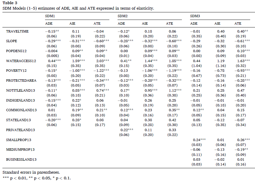
Protected areas – which in Bolivia are all based on co-management schemes - also protect forests in adjacent areas, showing an indirect protective spillover effect. Indigenous lands however only have direct forest protection effects.

Fischer et al. (2009)

The focus of this paper is on the role of human capital in explaining labor productivity variation among 198 European regions within a regression framework.

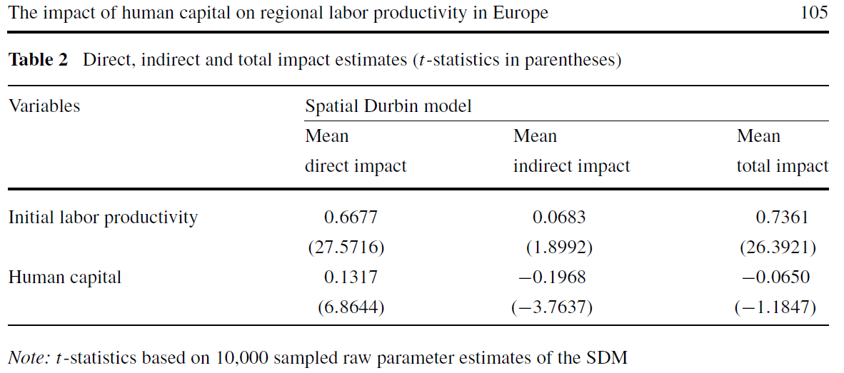
A ceteris paribus increase in the level of human capital is found to have a significant and positive direct impact. But this positive direct impact is offset by a significant and negative indirect (spillover) impact leading to a total impact that is not significantly different from zero.

The intuition here arises from the notion that it is relative regional advantages in human capital that matter most for labor productivity, so changing human capital across all regions should have little or no total impact on (average) labor productivity levels.

Rüttenauer (2018)

This study investigates the presence of environmental inequality in Germany - the connection between the presence of foreign-minority population and objectively measured industrial pollution.

Results reveal that the share of minorities within a census cell indeed positively correlates with the exposure to industrial pollution. Furthermore, spatial spillover effects are highly relevant: the characteristics of the neighbouring spatial units matter in predicting the amount of pollution. Especially within urban areas, clusters of high minority neighbourhoods are affected by high levels of environmental pollution.