7  Spatial Regression Models: Estimation

$$$$

This section is strongly based on Sarrias (2023), despite being much less detailed then the original.

Required packages

pkgs <- c("sf", "mapview", "spdep", "spatialreg", "tmap", "viridisLite") # note: load spdep first, then spatialreg
lapply(pkgs, require, character.only = TRUE)

Session info

sessionInfo()

R version 4.4.1 (2024-06-14 ucrt)
Platform: x86_64-w64-mingw32/x64
Running under: Windows 11 x64 (build 22631)

Matrix products: default


locale:
[1] LC_COLLATE=English_United Kingdom.utf8 
[2] LC_CTYPE=English_United Kingdom.utf8   
[3] LC_MONETARY=English_United Kingdom.utf8
[4] LC_NUMERIC=C                           
[5] LC_TIME=English_United Kingdom.utf8    

time zone: Europe/Berlin
tzcode source: internal

attached base packages:
[1] stats     graphics  grDevices utils     datasets  methods  
[7] base     

other attached packages:
[1] viridisLite_0.4.2 tmap_3.3-4        spatialreg_1.3-4 
[4] Matrix_1.7-0      spdep_1.3-5       spData_2.3.1     
[7] mapview_2.11.2    sf_1.0-16        

loaded via a namespace (and not attached):
 [1] xfun_0.45          raster_3.6-26      htmlwidgets_1.6.4 
 [4] lattice_0.22-6     tools_4.4.1        crosstalk_1.2.1   
 [7] LearnBayes_2.15.1  parallel_4.4.1     stats4_4.4.1      
[10] sandwich_3.1-0     proxy_0.4-27       KernSmooth_2.23-24
[13] satellite_1.0.5    RColorBrewer_1.1-3 leaflet_2.2.2     
[16] lifecycle_1.0.4    compiler_4.4.1     deldir_2.0-4      
[19] munsell_0.5.1      terra_1.7-78       codetools_0.2-20  
[22] leafsync_0.1.0     stars_0.6-5        htmltools_0.5.8.1 
[25] class_7.3-22       MASS_7.3-60.2      classInt_0.4-10   
[28] lwgeom_0.2-14      wk_0.9.1           abind_1.4-5       
[31] boot_1.3-30        multcomp_1.4-25    nlme_3.1-164      
[34] digest_0.6.35      mvtnorm_1.2-5      splines_4.4.1     
[37] fastmap_1.2.0      grid_4.4.1         colorspace_2.1-0  
[40] cli_3.6.2          magrittr_2.0.3     base64enc_0.1-3   
[43] dichromat_2.0-0.1  XML_3.99-0.16.1    survival_3.6-4    
[46] leafem_0.2.3       TH.data_1.1-2      e1071_1.7-14      
[49] scales_1.3.0       sp_2.1-4           rmarkdown_2.27    
[52] zoo_1.8-12         png_0.1-8          coda_0.19-4.1     
[55] evaluate_0.24.0    knitr_1.47         tmaptools_3.1-1   
[58] s2_1.1.6           rlang_1.1.4        Rcpp_1.0.12       
[61] glue_1.7.0         DBI_1.2.3          rstudioapi_0.16.0 
[64] jsonlite_1.8.8     R6_2.5.1           units_0.8-5       

Reload data from pervious session

load("_data/msoa2_spatial.RData")

Note that most of the spatial model specifications can not be estimated by Least Squares (LS), as using (constrained) LS estimators for models containing a spatially lagged dependent variable or disturbance leads to inconsistent results (Anselin and Bera 1998; Franzese and Hays 2007). However, an extensive amount of econometric literature discusses different estimation methods based on (quasi-) maximum likelihood (Anselin 1988; Lee 2004; Ord 1975) or instrumental variable approaches using generalized methods of moments (Drukker, Egger, and Prucha 2013; Kelejian and Prucha 1998, 2010), in which the endogenous lagged variables can be instrumented by $q$ higher order lags of the exogenous regressors $(\mathbf{X},\mathbf{W}\mathbf{X},{\mathbf{W}}^2\mathbf{X},...,{\mathbf{W}}^q\mathbf{X})$ (Kelejian and Prucha 1998).

7.1 Simulataneity bias

Remember what is happening when we estimate a spatial auto-regressive model.

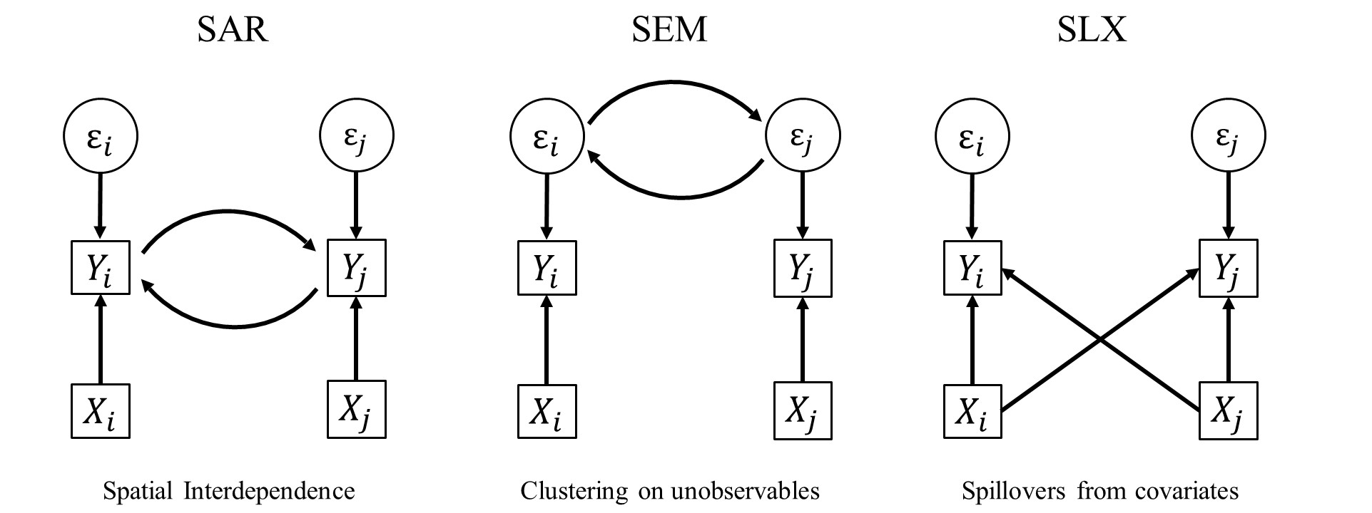
Note the circular process here: My $X$ influences my $Y$, which then influences your $Y$, which then influences my $Y$ again. We write this as

$$\mathbf{y}=\alpha \mathit{\iota }+\rho \mathbf{W}\mathbf{y}+\mathbf{X}\mathit{\beta }+\mathit{\epsilon }.$$

If we ignore $\mathbf{X}\mathit{\beta }$ and write the pure auto-regressive term in its reduce form, we get:

$$\mathbf{y}={({\mathbf{I}}_n-\rho \mathbf{W})}^{-1}\epsilon ,$$

and the spatial lag term is

$$\mathbf{W}\mathbf{y}=\mathbf{W}{({\mathbf{I}}_n-\rho \mathbf{W})}^{-1}\epsilon .$$

The OLS estimator for the spatial lag term then is

$${\hat{\rho }}_{OLS}={\left[\underset{(1\times n)}{\underbrace{{\left(\mathbf{W}\mathbf{y}\right)}^{⊺}}}\underset{(n\times 1)}{\underbrace{\left(\mathbf{W}\mathbf{y}\right)}}\right]}^{-1}\underset{(1\times n)}{\underbrace{{\left(\mathbf{W}\mathbf{y}\right)}^{⊺}}}\underset{(n\times 1)}{\underbrace{\mathbf{y}}}.$$

It can then be shown that the OLS estimators equals

$$\begin{gathered} {\hat{\rho }}_{OLS}=\rho +{\left[{\left(\mathbf{W}\mathbf{y}\right)}^{⊺}\left(\mathbf{W}\mathbf{y}\right)\right]}^{-1}{\left(\mathbf{W}\mathbf{y}\right)}^{⊺}\epsilon \\ =\rho +{\left(\sum _{i=1}^n{\mathbf{y}}_{Li}^2\right)}^{-1}\left(\sum _{i=1}^n{\mathbf{y}}_{Li}{ϵ}_i\right), \end{gathered}$$

with ${\mathbf{y}}_{Li}$ defined as the $i$th element of the spatial lag operator $\mathbf{W}\mathbf{y}={\mathbf{y}}_L$. It can further be shown that the second part of the equation $\ne 0$, which demonstrates that OLS gives a biased estimate of $\rho$ (Franzese and Hays 2007; Sarrias 2023).

Warning

Do not estimate spatial lags of the dependent variable in OLS. It will suffer from simultaneity bias.

7.2 Instrumental variable

A potential way of estimating spatial lag /SAR models is 2SLS (Kelejian and Prucha 1998).

We start with our standard model

$$\mathbf{y}=\alpha \mathit{\iota }+\rho \mathbf{W}\mathbf{y}+\mathbf{X}\mathit{\beta }+\mathit{\epsilon }.$$

As we have seen above, there is a problem of simultaneity: the “covariate” $\mathbf{W}\mathbf{y}$ is endogenous. One way of dealing with this endogeneity problem is the Instrumental Variable approach.

So, the question is what are good instruments $\mathbf{H}$ for $\mathbf{W}\mathbf{y}$? As we have specified the mode, we are sure that $\mathbf{X}$ determines $\mathbf{y}$. Thus, it must be true that $\mathbf{W}\mathbf{X}$ and ${\mathbf{W}}^2\mathbf{X},\dots ,{\mathbf{W}}^l\mathbf{X}$ determines $\mathbf{W}\mathbf{y}$.

Note that ${\mathbf{W}}^l$ denotes higher orders of $\mathbf{W}$. So ${\mathbf{W}}^2$ are the second order neighbours (neighbours of neighbours), and ${\mathbf{W}}^3$ are the third order neighbours (the neighbours of my neighbour’s neighbours), and so on…

We will discuss this in more detail later, but note for now that the reduced form of the SAR always contains a series of higher order neighbours.

$$({\mathbf{I}}_N-\rho \mathbf{W}{)}^{-1}{\beta }_k=({\mathbf{I}}_N+\rho \mathbf{W}+{\rho }^2{\mathbf{W}}^2+{\rho }^3{\mathbf{W}}^3+...){\beta }_k=({\mathbf{I}}_N+\sum _{h=1}^{\mathrm{\infty }}{\rho }^h{\mathbf{W}}^h){\beta }_k.$$

Thus, Kelejian and Prucha (1998) suggested to use a set of lagged covariates as instruments for $\mathbf{W}\mathbf{Y}$:

$$\mathbf{H}=\mathbf{X},\mathbf{W}\mathbf{X},{\mathbf{W}}^2\mathbf{X},...,{\mathbf{W}}^l\mathbf{X},$$

where $l$ is a pre-defined number for the higher order neighbours included. In practice, $l$ is usually restricted to $l=2$.

This has further been developed by, for instance, using a (truncated) power series as instruments (Kelejian, Prucha, and Yuzefovich 2004):

$$\mathbf{H}=[\mathbf{X},\mathbf{W}\left(\sum _{l=1}^{\mathrm{\infty }}{\rho }^l{\mathbf{W}}^l\right)\mathbf{X}\mathit{\beta }].$$

We can estimate this using the pacakge spatialreg with the function stsls(),

mod_1.sls <- stsls(log(med_house_price) ~ log(no2) + log(POPDEN) + 
                     per_mixed + per_asian + per_black + per_other,  
                   data = msoa.spdf, 
                   listw = queens.lw,
                   robust = TRUE, #  heteroskedasticity robust SEs
                   W2X = TRUE) # Second order neighbours are included as instruments (else only first)
summary(mod_1.sls)

Call:
stsls(formula = log(med_house_price) ~ log(no2) + log(POPDEN) + 
    per_mixed + per_asian + per_black + per_other, data = msoa.spdf, 
    listw = queens.lw, robust = TRUE, W2X = TRUE)

Residuals:
       Min         1Q     Median         3Q        Max 
-0.5464924 -0.1238002 -0.0052299  0.0989150  1.0793093 

Coefficients: 
               Estimate HC0 std. Error z value  Pr(>|z|)
Rho          0.71004211     0.04678235 15.1776 < 2.2e-16
(Intercept)  2.73582523     0.50997823  5.3646 8.113e-08
log(no2)     0.37752751     0.04920257  7.6729 1.688e-14
log(POPDEN) -0.05710992     0.01684036 -3.3913 0.0006957
per_mixed    0.01634307     0.00588488  2.7771 0.0054842
per_asian   -0.00205426     0.00045905 -4.4750 7.640e-06
per_black   -0.01166456     0.00128557 -9.0734 < 2.2e-16
per_other   -0.00280423     0.00332302 -0.8439 0.3987377

Residual variance (sigma squared): 0.035213, (sigma: 0.18765)

7.3 Generalized Method of Moments

Generalized Method of Moments (GMM) provides a way of estimating spatial error / SEM models. A motivation for GMM was that Maximum Likelihood was unfeasible for large samples and its consistent could not be shown. Kelejian and Prucha (1999) thus proposed a Moments estimator for SEM.

We start with the model

$$\begin{array}{rl}\mathbf{y}& =\alpha \mathit{\iota }+\mathbf{X}\mathit{\beta }+\mathbf{u},\\ \mathbf{u}& =\lambda \mathbf{W}\mathbf{u}+\mathit{\epsilon }\end{array}$$

The key issue here is to find a consistent estimator for $\lambda$. However, we usually do not want to draw inference about $\lambda$ itself, but only need it to consistently estimate $\mathit{\beta }$. Kelejian and Prucha (1999) thus treat $\lambda$ as pure nuisance parameter. They the following moment conditions:

$$\begin{array}{rl}\mathrm{E}\left[n^{-1}{\epsilon }^{⊺}\epsilon \right]& ={\sigma }^2,\\ \mathrm{E}\left[n^{-1}{\epsilon }^{⊺}\mathbf{W}\mathbf{W}\epsilon \right]& =\frac{{\sigma }^2}{n}\mathrm{E}[\mathrm{tr}({\mathbf{W}}^{⊺}\mathbf{W}\epsilon {\epsilon }^{⊺})],\\ \mathrm{E}\left[n^{-1}{\epsilon }^{⊺}\mathbf{W}\epsilon \right]& =0,\end{array}$$

which are solved for $\lambda$, ${\lambda }^2$, and ${\sigma }^2$ using $\epsilon =u-\lambda \mathbf{W}u$.

In essence, the GMM works as follows (Sarrias 2023):

1. First of all obtain a consistent estimate of $\mathit{\beta }$, say $\tilde{\mathit{\beta }}$ using either OLS or non-linear least squares (NLS).

2. Use this estimate to obtain an estimate of $\mathbf{u}$, say $\hat{\mathbf{u}}$,

3. Use $\hat{\mathbf{u}}$, to estimate $\lambda$, say $\hat{\lambda }$, using

$$({\hat{\lambda }}_{NLS,n},{\hat{\sigma }}_{NLS,N}^2)=\mathrm{argmin}\{{\mathit{\upsilon }}_n(\lambda ,{\sigma }^2{)}^{⊺}{\mathit{\upsilon }}_n(\lambda ,{\sigma }^2):\rho \in [-a,a],{\sigma }^2\in [0,b]\},$$

4. Estimate $\mathit{\beta }$ using Equation

$$\begin{array}{rl}{\mathit{\beta }}_{FGLS}(\lambda )& ={[{\mathbf{X}}^{⊺}\mathbf{\Omega }(\hat{\lambda }{)}^{-1}\mathbf{X}]}^{-1}{\mathbf{X}}^{⊺}\mathbf{\Omega }(\hat{\lambda }{)}^{-1}\mathbf{y}.\\ \mathbf{\Omega }(\lambda )& =(\mathbf{I}-\lambda \mathbf{W}{)}^{-1}(\mathbf{I}-\lambda {\mathbf{W}}^{⊺}{)}^{-1}\end{array}$$

For more, see for instance Kelejian and Piras (2017), chapter 2.2.4 or Sarrias (2023).

We can calculate the estimator using GMerrorsar() from spatialreg.

mod_1.gmm <- GMerrorsar(log(med_house_price) ~ log(no2) + log(POPDEN) + 
                     per_mixed + per_asian + per_black + per_other,  
                   data = msoa.spdf, 
                   listw = queens.lw,
                   se.lambda = TRUE) # Provide standard error for lambda
summary(mod_1.gmm)

Call:
GMerrorsar(formula = log(med_house_price) ~ log(no2) + log(POPDEN) + 
    per_mixed + per_asian + per_black + per_other, data = msoa.spdf, 
    listw = queens.lw, se.lambda = TRUE)

Residuals:
       Min         1Q     Median         3Q        Max 
-0.8275979 -0.1840855 -0.0096616  0.1610019  1.2270026 

Type: GM SAR estimator
Coefficients: (GM standard errors) 
               Estimate  Std. Error  z value  Pr(>|z|)
(Intercept) 11.07612114  0.26596129  41.6456 < 2.2e-16
log(no2)     0.67758095  0.08620995   7.8597 3.775e-15
log(POPDEN) -0.08006377  0.01464953  -5.4653 4.622e-08
per_mixed   -0.01307831  0.00894766  -1.4616    0.1438
per_asian   -0.00521983  0.00090937  -5.7400 9.465e-09
per_black   -0.01957288  0.00134527 -14.5494 < 2.2e-16
per_other   -0.00521695  0.00489760  -1.0652    0.2868

Lambda: 0.69344 (standard error): 0.071248 (z-value): 9.7328
Residual variance (sigma squared): 0.037126, (sigma: 0.19268)
GM argmin sigma squared: 0.037239
Number of observations: 983 
Number of parameters estimated: 9 

7.4 Maximum likelihood estimation

7.4.1 ML SAR

Maximum Likelihood estimation of spatial models is the most common way of estimation. The procedure to estimate Sar models via ML is based on Ord (1975) and Anselin (1988).

Starting with

$$\begin{array}{r}\mathbf{y}=\rho \mathbf{W}\mathbf{y}+\mathbf{X}\mathit{\beta }+\epsilon ,\\ \epsilon \sim \mathcal{N}({\mathbf{0}}_n,{\sigma }^2{\mathbf{I}}_n),\end{array}$$

and its reduced form

$$\begin{array}{r}\mathbf{y}=({\mathbf{I}}_N-\rho \mathbf{W}{)}^{-1}(\mathbf{X}\mathit{\beta }+\mathit{\epsilon }),\\ \mathbf{y}={\mathbf{A}}^{-1}(\mathbf{X}\mathit{\beta }+\mathit{\epsilon }),\end{array}$$

where $\mathbf{A}=({\mathbf{I}}_N-\rho \mathbf{W})$.

The ML estimator then choses the parameters $\hat{\rho }$, $\hat{\mathit{\beta }}$, and $\hat{\sigma }$ to maximize the probability of fitting the observed sample based on the Likelihood function

$$\begin{array}{rl}\mathcal{L}(\mathit{\theta })& =\log \left|\mathbf{A}\right|-\frac{n\log (2\pi )}{2}-\frac{n\log ({\sigma }^2)}{2}-\frac{1}{2{\sigma }^2}(\mathbf{A}\mathbf{y}-\mathbf{X}\mathit{\beta }{)}^{⊺}(\mathbf{A}\mathbf{y}-\mathbf{X}\mathit{\beta })\\ & =\log \left|\mathbf{A}\right|-\frac{n\log (2\pi )}{2}-\frac{n\log ({\sigma }^2)}{2}-\frac{1}{2{\sigma }^2}[{\mathbf{y}}^{⊺}{\mathbf{A}}^{⊺}\mathbf{A}\mathbf{y}-2{\left(\mathbf{A}\mathbf{y}\right)}^{⊺}\mathbf{X}\mathit{\beta }+{\mathit{\beta }}^{⊺}{\mathbf{X}}^{⊺}\mathbf{X}\mathit{\beta }],\end{array}$$

ML estimation of the SAR works as follows Sarrias (2023):

1. Perform the two auxiliary regression of $\mathbf{y}$ and $\mathbf{W}\mathbf{y}$ on $\mathbf{X}$ to obtain the estimators ${\hat{\mathit{\beta }}}_O$ and ${\hat{\mathit{\beta }}}_L$ as in Equation $$\begin{array}{rl}{\hat{\mathit{\beta }}}_{ML}(\rho )& ={\left({\mathbf{X}}^{⊺}\mathbf{X}\right)}^{-1}{\mathbf{X}}^{⊺}\mathbf{y}-\rho {\left({\mathbf{X}}^{⊺}\mathbf{X}\right)}^{-1}{\mathbf{X}}^{⊺}\mathbf{W}\mathbf{y},\\ & ={\hat{\mathit{\beta }}}_O-\rho {\hat{\mathit{\beta }}}_L.\end{array}$$

2. Use ${\hat{\mathit{\beta }}}_O$ and ${\hat{\mathit{\beta }}}_L$ to compute the residuals in Equation $${\epsilon }_O=\mathbf{y}-\mathbf{X}{\hat{\mathit{\beta }}}_0\text{and}{\epsilon }_L=\mathbf{W}\mathbf{y}-\mathbf{X}\widehat{{\mathit{\beta }}_L}.$$

3. By numerical optimization to obtain an estimate of $\rho$, maximize the concentrated likelihood given in

$$\ell (\rho )=-\frac{n}{2}-\frac{n}{2}\log (2\pi )-\frac{n}{2}\log \left[\frac{{({\epsilon }_O-\rho {\epsilon }_L)}^{⊺}({\epsilon }_O-\rho {\epsilon }_L)}{n}\right]+\log |{\mathbf{I}}_n-\rho \mathbf{W}|,$$

4. Use the estimate of $\hat{\rho }$ to plug it back in to the expression for $\mathit{\beta }$ and ${\sigma }^2$

$$\begin{array}{r}{\hat{\mathit{\beta }}}_{ML}(\rho )={\left({\mathbf{X}}^{⊺}\mathbf{X}\right)}^{-1}{\mathbf{X}}^{⊺}\mathbf{A}\mathbf{y}{\hat{\sigma }}_{ML}^2(\rho )=\\ \frac{{(\mathbf{A}\mathbf{y}-\mathbf{X}{\mathit{\beta }}_{ML})}^{⊺}(\mathbf{A}\mathbf{y}-\mathbf{X}{\mathit{\beta }}_{ML})}{n}\end{array}$$

The evaluation in step 3) can become computation burdensome, as each iteration involves the computation of the $N\times N$ Jacobian term $|{\mathbf{I}}_n-\rho \mathbf{W}|$. As shown by Ord (1975), this can be speeded up very heavily by using the log-determinant

$$\log |{\mathbf{I}}_n-\rho \mathbf{W}|=\sum _{i=1}^n\log (1-\rho {\omega }_i).$$

where ${\omega }_i$ are the eigenvalues of the weights matrix $\mathbf{W}$. The efficiency gains comes from the fact they also need to be calculated once. However, this requires $1-\rho {\omega }_i\ne 0$ or $1/{\omega }_{min}<\rho <1/{\omega }_{max}$. This can be ensures by normalising the weights matrix $\mathbf{W}$.

7.4.2 ML SEM

We can also use ML to estimate the spatial error / SEM model of the form

$$\begin{array}{rl}\mathbf{y}& =\alpha \mathit{\iota }+\mathbf{X}\mathit{\beta }+\mathbf{u},\\ \mathbf{u}& =\lambda \mathbf{W}\mathbf{u}+\mathit{\epsilon }\\ \epsilon & \sim \mathcal{N}({\mathbf{0}}_n,{\sigma }^2{\mathbf{I}}_n)\end{array}$$ Its reduce for is given by

$$\begin{array}{rl}\mathbf{y}& =\alpha \mathit{\iota }+\mathbf{X}\mathit{\beta }+({\mathbf{I}}_N-\lambda \mathbf{W}{)}^{-1}\mathit{\epsilon }.\\ \mathbf{y}& =\alpha \mathit{\iota }+\mathbf{X}\mathit{\beta }+{\mathbf{B}}^{-1}\mathit{\epsilon }.\end{array}$$

where $\mathbf{B}=({\mathbf{I}}_N-\lambda \mathbf{W})$.

Note that the OLS estimate of the SEM model are unbiased – if there is no omitted variable bias! However, even in that case, they are inefficient if $\lambda \ne 0$.

The log-likelihood function is given by

$$\begin{array}{r}\ell (\mathit{\theta })=-\frac{n}{2}\log (2\pi )-\frac{n}{2}\log ({\sigma }^2)-\frac{(\mathbf{y}-\mathbf{X}\mathit{\beta }{)}^{⊺}\mathbf{\Omega }(\lambda )(\mathbf{y}-\mathbf{X}\mathit{\beta })}{2{\sigma }^2}+\log |{\mathbf{I}}_n-\lambda \mathbf{W}|,\\ \mathbf{\Omega }(\lambda )={\mathbf{B}}^{⊺}\mathbf{B}={({\mathbf{I}}_n-\lambda \mathbf{W})}^{⊺}({\mathbf{I}}_n-\lambda \mathbf{W})\end{array}$$

Based on Anselin and Bera (1998), the ML estimation of SEM follow the procedure (Sarrias 2023):

1. Carry out an OLS of $\mathbf{B}\mathbf{X}$ on $\mathbf{B}\mathbf{y}$; get ${\hat{\mathit{\beta }}}_{OLS}$

2. Compute initial set of residuals ${\widehat{ϵ}}_{OLS}=\mathbf{B}\mathbf{y}-\mathbf{B}\mathbf{X}{\hat{\mathit{\beta }}}_{OLS}$

3. Given ${\widehat{ϵ}}_{OLS}$, find $\hat{\lambda }$ that maximizes the concentrated likelihood

$$\ell (\lambda )=\text{const}+\frac{n}{2}\log \left[\frac{1}{n}{\hat{\mathit{\epsilon }}}^{⊺}{\mathbf{B}}^{⊺}\mathbf{B}\hat{\mathit{\epsilon }}\right]+\log \left|\mathbf{B}\right|.$$

4. If the convergence criterion is met, proceed, otherwise repeat steps 1, 2 and 3.

5. Given $\hat{\lambda }$, estimate $\hat{\mathit{\beta }}(\lambda )$ by GLS and obtain a new vector of residuals, $\hat{\mathit{\epsilon }}(\lambda )$

6. Given $\hat{\mathit{\epsilon }}(\lambda )$ and $\hat{\lambda }$, estimate $\hat{\sigma }(\lambda )$.

The package spatialreg Pebesma and Bivand (2023) provides a series of functions to calculate the ML estimator for all spatial models we have considered.

Table from Pebesma and Bivand (2023):

model	model name	maximum likelihood estimation function
SEM	spatial error	errorsarlm(..., Durbin=FALSE)
SEM	spatial error	spautolm(..., family="SAR")
SDEM	spatial Durbin error	errorsarlm(..., Durbin=TRUE)
SLM	spatial lag	lagsarlm(..., Durbin=FALSE)
SDM	spatial Durbin	lagsarlm(..., Durbin=TRUE)
SAC	spatial autoregressive combined	sacsarlm(..., Durbin=FALSE)
GNM	general nested	sacsarlm(..., Durbin=TRUE)

ML SAR

mod_1.sar <- lagsarlm(log(med_house_price) ~ log(no2) + log(POPDEN) + 
                        per_mixed + per_asian + per_black + per_other,  
                      data = msoa.spdf, 
                      listw = queens.lw,
                      Durbin = FALSE) # we could here extend to SDM
summary(mod_1.sar)

Call:
lagsarlm(formula = log(med_house_price) ~ log(no2) + log(POPDEN) + 
    per_mixed + per_asian + per_black + per_other, data = msoa.spdf, 
    listw = queens.lw, Durbin = FALSE)

Residuals:
       Min         1Q     Median         3Q        Max 
-0.5281789 -0.1220524 -0.0099245  0.0992203  1.0936745 

Type: lag 
Coefficients: (asymptotic standard errors) 
               Estimate  Std. Error  z value  Pr(>|z|)
(Intercept)  3.17383180  0.29041604  10.9286 < 2.2e-16
log(no2)     0.39705423  0.04452880   8.9168 < 2.2e-16
log(POPDEN) -0.05583014  0.01242876  -4.4920 7.055e-06
per_mixed    0.01851577  0.00579832   3.1933  0.001407
per_asian   -0.00228346  0.00045876  -4.9775 6.442e-07
per_black   -0.01263650  0.00100282 -12.6009 < 2.2e-16
per_other   -0.00161419  0.00289082  -0.5584  0.576582

Rho: 0.66976, LR test value: 473.23, p-value: < 2.22e-16
Asymptotic standard error: 0.025311
    z-value: 26.461, p-value: < 2.22e-16
Wald statistic: 700.19, p-value: < 2.22e-16

Log likelihood: 196.7203 for lag model
ML residual variance (sigma squared): 0.035402, (sigma: 0.18815)
Number of observations: 983 
Number of parameters estimated: 9 
AIC: -375.44, (AIC for lm: 95.786)
LM test for residual autocorrelation
test value: 8.609, p-value: 0.0033451

ML SEM

mod_1.sem <- errorsarlm(log(med_house_price) ~ log(no2) + log(POPDEN) +
                          per_mixed + per_asian + per_black + per_other,  
                        data = msoa.spdf, 
                        listw = queens.lw,
                        Durbin = FALSE) # we could here extend to SDEM
summary(mod_1.sem)

Call:
errorsarlm(formula = log(med_house_price) ~ log(no2) + log(POPDEN) + 
    per_mixed + per_asian + per_black + per_other, data = msoa.spdf, 
    listw = queens.lw, Durbin = FALSE)

Residuals:
      Min        1Q    Median        3Q       Max 
-0.581785 -0.105218 -0.012758  0.094430  0.913425 

Type: error 
Coefficients: (asymptotic standard errors) 
               Estimate  Std. Error  z value  Pr(>|z|)
(Intercept) 12.92801104  0.35239139  36.6865 < 2.2e-16
log(no2)     0.15735296  0.10880727   1.4462 0.1481317
log(POPDEN) -0.08316270  0.01254315  -6.6301 3.354e-11
per_mixed   -0.03377962  0.00811054  -4.1649 3.115e-05
per_asian   -0.00413115  0.00096849  -4.2656 1.994e-05
per_black   -0.01653816  0.00126741 -13.0488 < 2.2e-16
per_other   -0.01693012  0.00462999  -3.6566 0.0002556

Lambda: 0.88605, LR test value: 623.55, p-value: < 2.22e-16
Asymptotic standard error: 0.015803
    z-value: 56.068, p-value: < 2.22e-16
Wald statistic: 3143.6, p-value: < 2.22e-16

Log likelihood: 271.8839 for error model
ML residual variance (sigma squared): 0.026911, (sigma: 0.16405)
Number of observations: 983 
Number of parameters estimated: 9 
AIC: -525.77, (AIC for lm: 95.786)

Anselin, Luc. 1988. Spatial Econometrics: Methods and Models. Studies in Operational Regional Science. Dordrecht: Kluwer.

Anselin, Luc, and Anil K. Bera. 1998. “Spatial Dependence in Linear Regression Models with an Introduction to Spatial Econometrics.” In Handbook of Applied Economic Statistics, edited by Aman Ullah and David E. A. Giles, 237–89. New York: Dekker.

Bivand, Roger, Giovanni Millo, and Gianfranco Piras. 2021. “A Review of Software for Spatial Econometrics in R.” Mathematics 9 (11): 1276. https://doi.org/10.3390/math9111276.

Drukker, David M., Peter Egger, and Ingmar R. Prucha. 2013. “On Two-Step Estimation of a Spatial Autoregressive Model with Autoregressive Disturbances and Endogenous Regressors.” Econometric Reviews 32 (5-6): 686–733. https://doi.org/10.1080/07474938.2013.741020.

Franzese, Robert J., and Jude C. Hays. 2007. “Spatial Econometric Models of Cross-Sectional Interdependence in Political Science Panel and Time-Series-Cross-Section Data.” Political Analysis 15 (2): 140–64. https://doi.org/10.1093/pan/mpm005.

Kelejian, Harry H., and Gianfranco Piras. 2017. Spatial Econometrics. Elsevier. https://doi.org/10.1016/C2016-0-04332-2.

Kelejian, Harry H., and Ingmar R. Prucha. 1998. “A Generalized Spatial Two-Stage Least Squares Procedure for Estimating a Spatial Autoregressive Model with Autoregressive Disturbances.” The Journal of Real Estate Finance and Economics 17 (1): 99–121. https://doi.org/10.1023/A:1007707430416.

———. 1999. “A Generalized Moments Estimator for the Autoregressive Parameter in a Spatial Model.” International Economic Review 40 (2): 509–33. https://doi.org/10.1111/1468-2354.00027.

———. 2010. “Specification and Estimation of Spatial Autoregressive Models with Autoregressive and Heteroskedastic Disturbances.” Journal of Econometrics 157 (1): 53–67. https://doi.org/10.1016/j.jeconom.2009.10.025.

Kelejian, Harry H., Ingmar R. Prucha, and Yevgeny Yuzefovich. 2004. “Instrumental Variable Estimation of a Spatial Autoregressive Model with Autoregressive Disturbances: Large and Small Sample Results.” In Spatial and Spatiotemporal Econometrics, edited by James P. LeSage and R. Kelley Pace, 163–98. Advances in Econometrics. Amsterdam and Boston: Elsevier.

Lee, Lung-fei. 2004. “Asymptotic Distributions of Quasi-Maximum Likelihood Estimators for Spatial Autoregressive Models.” Econometrica 72 (6): 1899–1925.

Ord, John Keith. 1975. “Estimation Methods for Models of Spatial Interaction.” Journal of the American Statistical Association 70 (349): 120–26. https://doi.org/10.2307/2285387.

Pebesma, Edzer, and Roger Bivand. 2023. Spatial Data Science: With Applications in R. First. Boca Raton: Chapman and Hall/CRC. https://doi.org/10.1201/9780429459016.

Sarrias, Mauricio. 2023. Intermediate Spatial Econometrics with Applications in R.