10  Spatio-temporal models

Required packages

pkgs <- c("sf", "mapview", "spdep", "spatialreg", "tmap", "viridisLite", 
          "plm", "splm", "SDPDmod")
lapply(pkgs, require, character.only = TRUE)

Session info

sessionInfo()

R version 4.3.1 (2023-06-16 ucrt)
Platform: x86_64-w64-mingw32/x64 (64-bit)
Running under: Windows 10 x64 (build 19044)

Matrix products: default


locale:
[1] LC_COLLATE=English_United Kingdom.utf8 
[2] LC_CTYPE=English_United Kingdom.utf8   
[3] LC_MONETARY=English_United Kingdom.utf8
[4] LC_NUMERIC=C                           
[5] LC_TIME=English_United Kingdom.utf8    

time zone: Europe/London
tzcode source: internal

attached base packages:
[1] stats     graphics  grDevices utils     datasets  methods  
[7] base     

other attached packages:
 [1] SDPDmod_0.0.3     splm_1.6-2        plm_2.6-3        
 [4] viridisLite_0.4.2 tmap_3.3-3        spatialreg_1.2-9 
 [7] Matrix_1.5-4.1    spdep_1.2-8       spData_2.2.2     
[10] mapview_2.11.0    sf_1.0-13        

loaded via a namespace (and not attached):
 [1] tidyselect_1.2.0   dplyr_1.1.2        fastmap_1.1.1     
 [4] leaflet_2.1.2      TH.data_1.1-2      dotCall64_1.0-2   
 [7] XML_3.99-0.14      digest_0.6.31      lifecycle_1.0.3   
[10] LearnBayes_2.15.1  survival_3.5-5     terra_1.7-29      
[13] magrittr_2.0.3     compiler_4.3.1     rlang_1.1.1       
[16] tools_4.3.1        utf8_1.2.3         collapse_1.9.6    
[19] knitr_1.43         htmlwidgets_1.6.2  sp_1.6-1          
[22] classInt_0.4-9     RColorBrewer_1.1-3 multcomp_1.4-24   
[25] abind_1.4-5        KernSmooth_2.23-21 expm_0.999-7      
[28] leafsync_0.1.0     grid_4.3.1         stats4_4.3.1      
[31] fansi_1.0.4        xtable_1.8-4       lfe_2.9-0         
[34] e1071_1.7-13       leafem_0.2.0       colorspace_2.1-0  
[37] scales_1.2.1       MASS_7.3-60        dichromat_2.0-0.1 
[40] cli_3.6.1          mvtnorm_1.2-2      rmarkdown_2.22    
[43] miscTools_0.6-28   generics_0.1.3     RSpectra_0.16-1   
[46] rstudioapi_0.14    tmaptools_3.1-1    bdsmatrix_1.3-6   
[49] DBI_1.1.3          proxy_0.4-27       ibdreg_0.3.8      
[52] splines_4.3.1      stars_0.6-1        parallel_4.3.1    
[55] s2_1.1.4           base64enc_0.1-3    vctrs_0.6.3       
[58] boot_1.3-28.1      webshot_0.5.4      sandwich_3.0-2    
[61] jsonlite_1.8.5     Formula_1.2-5      crosstalk_1.2.0   
[64] units_0.8-2        spam_2.9-1         glue_1.6.2        
[67] lwgeom_0.2-13      codetools_0.2-19   deldir_1.0-9      
[70] raster_3.6-20      lmtest_0.9-40      munsell_0.5.0     
[73] tibble_3.2.1       pillar_1.9.0       htmltools_0.5.5   
[76] satellite_1.0.4    R6_2.5.1           maxLik_1.5-2      
[79] wk_0.7.3           Rdpack_2.4         evaluate_0.21     
[82] lattice_0.21-8     rbibutils_2.2.13   png_0.1-8         
[85] class_7.3-22       Rcpp_1.0.10        coda_0.19-4       
[88] nlme_3.1-162       xfun_0.39          zoo_1.8-12        
[91] pkgconfig_2.0.3   

Elhorst (2014) provides a comprehensive introduction to spatial panel data methods. Article length introduction to spatial panel data models (FE and RE) can be found in Elhorst (2012), Millo and Piras (2012) and Croissant and Millo (2018). LeSage (2014) discusses Bayesian panel data methods.

Note that we will only discuss some basics here, as the complete econometrics of these models and their estimation strategy become insanely complicated (Lee and Yu 2010).

10.1 Static panel data models

The idea behind a static panel data with auto-regressive term is similar to the cross sectional situation (Millo and Piras 2012).

\[ {\boldsymbol{\mathbf{y}}}= \rho(\boldsymbol{\mathbf{I}}_T\otimes {\boldsymbol{\mathbf{W}}_N}){\boldsymbol{\mathbf{y}}}+{\boldsymbol{\mathbf{X}}}{\boldsymbol{\mathbf{\beta}}}+ {\boldsymbol{\mathbf{u}}}. \]

where \(\otimes\) is the Kronecker product (block-wise multiplication).

\[ \begin{split} \underbrace{\underbrace{\boldsymbol{\mathbf{I}}_T}_{T \times T} \otimes \underbrace{\boldsymbol{\mathbf{W}}_N}_{N \times N}}_{NT \times NT}= \begin{pmatrix} 1 & 0 & \cdots & 0 \\ 0 & 1 & \cdots & 0 \\ \vdots & \vdots & \ddots & \vdots \\ 0 & 0 & \cdots & 1 \end{pmatrix} \left[\begin{array}{cccc} v_{1} w_{1} & v_{1} w_{2} & \cdots & v_{1} w_{m} \\ v_{2} w_{1} & v_{2} w_{2} & \cdots & v_{2} w_{m} \\ \vdots & \vdots & \ddots & \vdots \\ v_{n} w_{1} & v_{n} w_{2} & \cdots & v_{n} w_{m} \end{array}\right] =\\ \begin{pmatrix} \left[\begin{array}{cccc} v_{1} w_{1} & v_{1} w_{2} & \cdots & v_{1} w_{m} \\ v_{2} w_{1} & v_{2} w_{2} & \cdots & v_{2} w_{m} \\ \vdots & \vdots & \ddots & \vdots \\ v_{n} w_{1} & v_{n} w_{2} & \cdots & v_{n} w_{m} \end{array}\right] & 0 & \cdots & 0 \\ 0 & \left[\begin{array}{cccc} v_{1} w_{1} & v_{1} w_{2} & \cdots & v_{1} w_{m} \\ v_{2} w_{1} & v_{2} w_{2} & \cdots & v_{2} w_{m} \\ \vdots & \vdots & \ddots & \vdots \\ v_{n} w_{1} & v_{n} w_{2} & \cdots & v_{n} w_{m} \end{array}\right] & \cdots & 0 \\ \vdots & \vdots & \ddots & \vdots \\ 0 & 0 & \cdots & \left[\begin{array}{cccc} v_{1} w_{1} & v_{1} w_{2} & \cdots & v_{1} w_{m} \\ v_{2} w_{1} & v_{2} w_{2} & \cdots & v_{2} w_{m} \\ \vdots & \vdots & \ddots & \vdots \\ v_{n} w_{1} & v_{n} w_{2} & \cdots & v_{n} w_{m} \end{array}\right] \end{pmatrix} \end{split} \]

Here we model only spatial dependence within each cross-section and multiply the same spatial weights matrix \(T\) times. Off block-diagonal elements are all zero. So there is no spatial dependence that goes across time.

The error term can be decomposed into two parts:

\[ {\boldsymbol{\mathbf{u}}}= (\boldsymbol{\mathbf{\iota}}_T \otimes {\boldsymbol{\mathbf{I}}_N})\boldsymbol{\mathbf{\mu}}+ {\boldsymbol{\mathbf{\nu}}}, \]

where \(\boldsymbol{\mathbf{\iota}}_T\) is a \(T \times 1\) vector of ones, \({\boldsymbol{\mathbf{I}}_N}\) an \(N \times N\) identity matrix, \(\boldsymbol{\mathbf{\mu}}\) is a vector of time-invariant individual specific effects (not spatially autocorrelated).

We could obviously extent the specification to allow for error correlation by specifying

\[ {\boldsymbol{\mathbf{\nu}}}= \lambda(\boldsymbol{\mathbf{I}}_T \otimes {\boldsymbol{\mathbf{W}}_N})\boldsymbol{\mathbf{\nu }}+ {\boldsymbol{\mathbf{\varepsilon}}}. \]

The individual effects can be treated as fixed or random.

Fixed Effects

In the FE model, the individual specific effects are treated as fixed. If we re-write the equation above, we derive at the well-know fixed effects formula with an additional spatial autoregressive term:

\[ {y_{it}}= \rho\sum_{j=1}^Nw_{ij}y_{jt} + \boldsymbol{\mathbf{x}}_{it}\boldsymbol{\mathbf{\beta }}+ \mu_i + \nu_{it}, \] where \(\mu_i\) denote the individual-specific fixed effects.

As with the standard spatial lag model, we cannot rely on the OLS estimator because of the simultaneity problem. The coefficients are thus estimated by maximum likelihood (Elhorst 2014).

Random Effects

In the RE model, the individual specific effects are treated as components of the error \(\mu \sim \mathrm{IID}(o, \sigma_\mu^2)\). The model can then be written as

\[ \begin{split} {\boldsymbol{\mathbf{y}}}= \rho(\boldsymbol{\mathbf{I}}_T\otimes {\boldsymbol{\mathbf{W}}_N}){\boldsymbol{\mathbf{y}}}+{\boldsymbol{\mathbf{X}}}{\boldsymbol{\mathbf{\beta}}}+ {\boldsymbol{\mathbf{u}}}, \\ {\boldsymbol{\mathbf{u}}}= (\boldsymbol{\mathbf{\iota}}_T \otimes {\boldsymbol{\mathbf{I}}_N})\boldsymbol{\mathbf{\mu}}+ [\boldsymbol{\mathbf{I}}_T \otimes (\boldsymbol{\mathbf{I}}_N - \lambda{\boldsymbol{\mathbf{W}}_N})]^{-1} {\boldsymbol{\mathbf{\varepsilon}}}. \end{split} \]

As with the conventional random effects model, we make the strong assumption that the unobserved individual effects are uncorrelated with the covariates \(\boldsymbol{\mathbf{X}}\) in the model.

10.2 Dynamic panel data models

Relying on panel data and repeated measures over time, comes with an additional layer of dependence / autocorrelation between units. We have spatial dependence (with its three potential sources), and we have temporal/serial dependence within each unit over time.

A general dynamic model would account for all sources of potential dependence, including combinations (Elhorst 2012). The most general model can be written as:

\[ \begin{split} {\boldsymbol{\mathbf{y}}_t}=& \tau \boldsymbol{\mathbf{y}}_{t-1} + \rho(\boldsymbol{\mathbf{I}}_T\otimes {\boldsymbol{\mathbf{W}}_N}){\boldsymbol{\mathbf{y}}}_t + \gamma(\boldsymbol{\mathbf{I}}_T\otimes {\boldsymbol{\mathbf{W}}_N}){\boldsymbol{\mathbf{y}}_{t-1}}\\ &~+ {\boldsymbol{\mathbf{X}}}{\boldsymbol{\mathbf{\beta}}}+ (\boldsymbol{\mathbf{I}}_T\otimes {\boldsymbol{\mathbf{W}}_N}){\boldsymbol{\mathbf{X}}}{\boldsymbol{\mathbf{\theta}}}+ {\boldsymbol{\mathbf{u}}}_t,\\ {\boldsymbol{\mathbf{u}}_t}=& + (\boldsymbol{\mathbf{\iota}}_T \otimes {\boldsymbol{\mathbf{I}}_N})\boldsymbol{\mathbf{\mu}}+ {\boldsymbol{\mathbf{\nu}}_t},\\ {\boldsymbol{\mathbf{\nu}}_t}=& \psi{\boldsymbol{\mathbf{\nu}}}_{t-1} + \lambda(\boldsymbol{\mathbf{I}}_T \otimes {\boldsymbol{\mathbf{W}}_N})\boldsymbol{\mathbf{\nu }}+ {\boldsymbol{\mathbf{\varepsilon}}}, \end{split} \]

Where \({\boldsymbol{\mathbf{X}}}\) could further contain time-lagged covariates. Compared to the static spatial panel model, we have introduced temporal dependency in the outcome \(\tau \boldsymbol{\mathbf{y}}_{t-1}\) and the spatially lagged outcome \(\gamma(\boldsymbol{\mathbf{I}}_T\otimes {\boldsymbol{\mathbf{W}}_N}){\boldsymbol{\mathbf{y}}_{t-1}}\), and in the error term \(\psi{\boldsymbol{\mathbf{\nu}}}_{t-1}\).

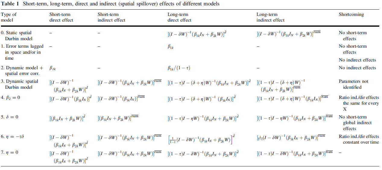
10.2.1 Impacts in spatial panel models

Note that similar to the distinction between local and global spillovers, we now have to distinguish between short-term and long-term effects. A change in \(\boldsymbol{\mathbf{X}}_t\) no influences focal \(Y\) and neighbour’s \(Y\) but also contemporaneous \(Y\) and future \(Y\).

While the short-term effects are the known impacts

\[ \frac{\partial {\boldsymbol{\mathbf{y}}}}{\partial {\boldsymbol{\mathbf{x}}}_k} = ({\boldsymbol{\mathbf{I}}}-\rho{\boldsymbol{\mathbf{W}}_{NT}})^{-1}\left[\beta_k+{\boldsymbol{\mathbf{W}}_{NT}}\theta_k\right]. \]

The long-term impacts, by contrast, additionally account for the effect multiplying through time

\[ \frac{\partial {\boldsymbol{\mathbf{y}}}}{\partial {\boldsymbol{\mathbf{x}}}_k} = [(1-\tau){\boldsymbol{\mathbf{I}}}-(\rho+\gamma){\boldsymbol{\mathbf{W}}_{NT}}]^{-1}\left[\beta_k+{\boldsymbol{\mathbf{W}}_{NT}}\theta_k\right]. \]

For more information see Elhorst (2012).

Summary impact measures in dynamic spatial panel models (Elhorst 2012)

10.3 Example: Local employment impacts of immigration

Fingleton, Olner, and Pryce (2020): Estimating the local employment impacts of immigration: A dynamic spatial panel model. Urban Studies, 57(13), 2646–2662. https://doi.org/10.1177/0042098019887916

This paper highlights a number of important gaps in the UK evidence base on the employment impacts of immigration, namely: (1) the lack of research on the local impacts of immigration – existing studies only estimate the impact for the country as a whole; (2) the absence of long-term estimates – research has focused on relatively short time spans – there are no estimates of the impact over several decades, for example; (3) the tendency to ignore spatial dependence of employment which can bias the results and distort inference – there are no robust spatial econometric estimates we are aware of.

We illustrate our approach with an application to London and find that no migrant group has a statistically significant long-term negative effect on employment. EU migrants, however, are found to have a significant positive impact, which may have important implications for the Brexit debate. Our approach opens up a new avenue of inquiry into subnational variations in the impacts of immigration on employment.

Impacts on employment, Fingleton, Olner, and Pryce (2020)

10.4 Estimation in R

To estimate spatial panel models in R, we can use the splm package of Millo and Piras (2012).

We use a standard example with longitudinal data from the plm package here.

data(Produc, package = "plm")
data(usaww)

head(Produc)

    state year region     pcap     hwy   water    util       pc
1 ALABAMA 1970      6 15032.67 7325.80 1655.68 6051.20 35793.80
2 ALABAMA 1971      6 15501.94 7525.94 1721.02 6254.98 37299.91
3 ALABAMA 1972      6 15972.41 7765.42 1764.75 6442.23 38670.30
4 ALABAMA 1973      6 16406.26 7907.66 1742.41 6756.19 40084.01
5 ALABAMA 1974      6 16762.67 8025.52 1734.85 7002.29 42057.31
6 ALABAMA 1975      6 17316.26 8158.23 1752.27 7405.76 43971.71
    gsp    emp unemp
1 28418 1010.5   4.7
2 29375 1021.9   5.2
3 31303 1072.3   4.7
4 33430 1135.5   3.9
5 33749 1169.8   5.5
6 33604 1155.4   7.7

usaww[1:10, 1:10]

            ALABAMA   ARIZONA ARKANSAS CALIFORNIA COLORADO
ALABAMA         0.0 0.0000000        0        0.0      0.0
ARIZONA         0.0 0.0000000        0        0.2      0.2
ARKANSAS        0.0 0.0000000        0        0.0      0.0
CALIFORNIA      0.0 0.3333333        0        0.0      0.0
COLORADO        0.0 0.1428571        0        0.0      0.0
CONNECTICUT     0.0 0.0000000        0        0.0      0.0
DELAWARE        0.0 0.0000000        0        0.0      0.0
FLORIDA         0.5 0.0000000        0        0.0      0.0
GEORGIA         0.2 0.0000000        0        0.0      0.0
IDAHO           0.0 0.0000000        0        0.0      0.0
            CONNECTICUT DELAWARE FLORIDA GEORGIA IDAHO
ALABAMA               0        0    0.25    0.25     0
ARIZONA               0        0    0.00    0.00     0
ARKANSAS              0        0    0.00    0.00     0
CALIFORNIA            0        0    0.00    0.00     0
COLORADO              0        0    0.00    0.00     0
CONNECTICUT           0        0    0.00    0.00     0
DELAWARE              0        0    0.00    0.00     0
FLORIDA               0        0    0.00    0.50     0
GEORGIA               0        0    0.20    0.00     0
IDAHO                 0        0    0.00    0.00     0

Produc contains data on US States Production - a panel of 48 observations from 1970 to 1986. usaww is a spatial weights matrix of the 48 continental US States based on the queen contiguity relation.

Let start with an FE SEM model, using function spml() for maximum likelihood estimation of static spatial panel models.

# Gen listw object
usalw <- mat2listw(usaww, style = "W")

# Spec formula
fm <- log(gsp) ~ log(pcap) + log(pc) + log(emp) + unemp

### Esimate FE SEM model
semfe.mod <- spml(formula = fm, data = Produc, 
                  index = c("state", "year"),  # ID column
                  listw = usalw,          # listw
                  model = "within",       # one of c("within", "random", "pooling").
                  effect = "individual",  # type of fixed effects
                  lag = FALSE,            # spatila lg of Y
                  spatial.error = "b",    # "b" (Baltagi), "kkp" (Kapoor, Kelejian and Prucha)
                  method = "eigen",       # estimation method, for large data e.g. ("spam", "Matrix" or "LU")
                  na.action = na.fail,    # handling of missings
                  zero.policy = NULL)     # handling of missings

summary(semfe.mod)

Spatial panel fixed effects error model
 

Call:
spml(formula = fm, data = Produc, index = c("state", "year"), 
    listw = usalw, na.action = na.fail, model = "within", effect = "individual", 
    lag = FALSE, spatial.error = "b", method = "eigen", zero.policy = NULL)

Residuals:
      Min.    1st Qu.     Median    3rd Qu.       Max. 
-0.1246945 -0.0237699 -0.0034993  0.0170886  0.1882224 

Spatial error parameter:
    Estimate Std. Error t-value  Pr(>|t|)    
rho 0.557401   0.033075  16.853 < 2.2e-16 ***

Coefficients:
            Estimate Std. Error t-value Pr(>|t|)    
log(pcap)  0.0051438  0.0250109  0.2057  0.83705    
log(pc)    0.2053026  0.0231427  8.8712  < 2e-16 ***
log(emp)   0.7822540  0.0278057 28.1328  < 2e-16 ***
unemp     -0.0022317  0.0010709 -2.0839  0.03717 *  
---
Signif. codes:  0 '***' 0.001 '**' 0.01 '*' 0.05 '.' 0.1 ' ' 1

A RE SAR model, by contrast, can be estimated using the following options:

### Estimate an RE SAR model
sarre.mod <- spml(formula = fm, data = Produc, 
                  index = c("state", "year"),  # ID column
                  listw = usalw,          # listw
                  model = "random",       # one of c("within", "random", "pooling").
                  effect = "individual",  # type of fixed effects
                  lag = TRUE,             # spatila lg of Y
                  spatial.error = "none", # "b" (Baltagi), "kkp" (Kapoor, Kelejian and Prucha)
                  method = "eigen",       # estimation method, for large data e.g. ("spam", "Matrix" or "LU")
                  na.action = na.fail,    # handling of missings
                  zero.policy = NULL)     # handling of missings

summary(sarre.mod)

ML panel with spatial lag, random effects 

Call:
spreml(formula = formula, data = data, index = index, w = listw2mat(listw), 
    w2 = listw2mat(listw2), lag = lag, errors = errors, cl = cl, 
    method = "eigen", zero.policy = ..2)

Residuals:
   Min. 1st Qu.  Median    Mean 3rd Qu.    Max. 
   1.38    1.57    1.70    1.70    1.80    2.13 

Error variance parameters:
    Estimate Std. Error t-value Pr(>|t|)  
phi  21.3175     8.2929  2.5706  0.01015 *

Spatial autoregressive coefficient:
       Estimate Std. Error t-value  Pr(>|t|)    
lambda 0.161615   0.029042  5.5648 2.625e-08 ***

Coefficients:
               Estimate  Std. Error t-value  Pr(>|t|)    
(Intercept)  1.65814987  0.15071855 11.0016 < 2.2e-16 ***
log(pcap)    0.01294505  0.02493997  0.5190    0.6037    
log(pc)      0.22555375  0.02163422 10.4258 < 2.2e-16 ***
log(emp)     0.67081074  0.02642113 25.3892 < 2.2e-16 ***
unemp       -0.00579716  0.00089175 -6.5009 7.984e-11 ***
---
Signif. codes:  0 '***' 0.001 '**' 0.01 '*' 0.05 '.' 0.1 ' ' 1

Note that Millo and Piras (2012) use a different notation, namely \(\lambda\) for lag dependence, and \(\rho\) for error dependence….

Again, we have to use an additional step to get impacts for SAR-like models.

# Number of years
T <- length(unique(Produc$year))

# impacts
sarre.mod.imp <- impacts(sarre.mod,
                         listw = usalw,
                         time = T)
summary(sarre.mod.imp)                         

Impact measures (lag, trace):
                Direct     Indirect        Total
log(pcap)  0.013028574  0.002411880  0.015440454
log(pc)    0.227009032  0.042024438  0.269033470
log(emp)   0.675138835  0.124983264  0.800122098
unemp     -0.005834562 -0.001080108 -0.006914669
========================================================
Simulation results ( variance matrix):
Direct:

Iterations = 1:200
Thinning interval = 1 
Number of chains = 1 
Sample size per chain = 200 

1. Empirical mean and standard deviation for each variable,
   plus standard error of the mean:

               Mean        SD  Naive SE Time-series SE
log(pcap)  0.014018 0.0269148 1.903e-03      1.903e-03
log(pc)    0.229110 0.0217812 1.540e-03      1.540e-03
log(emp)   0.672171 0.0279965 1.980e-03      1.980e-03
unemp     -0.005876 0.0009191 6.499e-05      6.499e-05

2. Quantiles for each variable:

               2.5%       25%       50%       75%     97.5%
log(pcap) -0.040735 -0.002110  0.014639  0.031085  0.064264
log(pc)    0.189454  0.213645  0.228699  0.243676  0.274472
log(emp)   0.617315  0.653580  0.671957  0.692865  0.728716
unemp     -0.007725 -0.006416 -0.005892 -0.005249 -0.004214

========================================================
Indirect:

Iterations = 1:200
Thinning interval = 1 
Number of chains = 1 
Sample size per chain = 200 

1. Empirical mean and standard deviation for each variable,
   plus standard error of the mean:

               Mean        SD  Naive SE Time-series SE
log(pcap)  0.002625 0.0051289 3.627e-04      3.627e-04
log(pc)    0.043037 0.0098790 6.986e-04      6.986e-04
log(emp)   0.125961 0.0247641 1.751e-03      1.751e-03
unemp     -0.001102 0.0002789 1.972e-05      2.191e-05

2. Quantiles for each variable:

               2.5%        25%       50%       75%      97.5%
log(pcap) -0.007588 -0.0003474  0.002949  0.005978  0.0120732
log(pc)    0.026912  0.0358375  0.042576  0.049154  0.0618856
log(emp)   0.078987  0.1074866  0.125531  0.142507  0.1744827
unemp     -0.001636 -0.0012761 -0.001077 -0.000920 -0.0006084

========================================================
Total:

Iterations = 1:200
Thinning interval = 1 
Number of chains = 1 
Sample size per chain = 200 

1. Empirical mean and standard deviation for each variable,
   plus standard error of the mean:

               Mean       SD  Naive SE Time-series SE
log(pcap)  0.016644 0.031958 2.260e-03      2.260e-03
log(pc)    0.272147 0.028217 1.995e-03      1.995e-03
log(emp)   0.798132 0.040933 2.894e-03      2.894e-03
unemp     -0.006978 0.001114 7.879e-05      7.879e-05

2. Quantiles for each variable:

              2.5%       25%       50%       75%     97.5%
log(pcap) -0.04982 -0.002483  0.017731  0.036710  0.077099
log(pc)    0.22333  0.251301  0.270158  0.291200  0.334917
log(emp)   0.71769  0.768460  0.796217  0.826540  0.875376
unemp     -0.00910 -0.007736 -0.006924 -0.006279 -0.005004

There is an alternative by using the package SDPDmod by Rozeta Simonovska (see vignette).

### FE SAR model
sarfe.mod2 <- SDPDm(formula = fm, 
                    data = Produc, 
                    W = usaww,                 
                    index = c("state","year"), # ID
                    model = "sar",             # on of c("sar","sdm"),
                    effect = "individual",     # FE structure
                    dynamic = FALSE,           # time lags of the dependet variable
                    LYtrans = TRUE)            # Lee-Yu transformation (bias correction)

summary(sarfe.mod2)

sar panel model with individual fixed effects

Call:
SDPDm(formula = fm, data = Produc, W = usaww, index = c("state", 
    "year"), model = "sar", effect = "individual", dynamic = FALSE, 
    LYtrans = TRUE)

Spatial autoregressive coefficient:
    Estimate Std. Error t-value  Pr(>|t|)    
rho 0.278598   0.023999  11.609 < 2.2e-16 ***

Coefficients:
            Estimate Std. Error t-value  Pr(>|t|)    
log(pcap) -0.0468727  0.0262162 -1.7879   0.07379 .  
log(pc)    0.1859441  0.0237251  7.8374 4.598e-15 ***
log(emp)   0.6230539  0.0305554 20.3910 < 2.2e-16 ***
unemp     -0.0044700  0.0008917 -5.0129 5.362e-07 ***
---
Signif. codes:  0 '***' 0.001 '**' 0.01 '*' 0.05 '.' 0.1 ' ' 1

And subsequently, we can calculate the impacts of the model.

# Impats
sarfe.mod2.imp <- impactsSDPDm(sarfe.mod2, 
                               NSIM = 200, # N simulations
                               sd = 12345) # seed

summary(sarfe.mod2.imp)

Impact estimates for spatial (static) model
========================================================

Direct:
             Estimate  Std. Error t-value  Pr(>|t|)    
log(pcap) -0.04549036  0.02599130 -1.7502   0.08008 .  
log(pc)    0.18809827  0.02383588  7.8914 2.988e-15 ***
log(emp)   0.63773076  0.03027063 21.0676 < 2.2e-16 ***
unemp     -0.00459914  0.00089696 -5.1275 2.936e-07 ***

Indirect:
             Estimate  Std. Error t-value  Pr(>|t|)    
log(pcap) -0.01635880  0.00940186 -1.7400   0.08187 .  
log(pc)    0.06724675  0.00991019  6.7856 1.156e-11 ***
log(emp)   0.22820595  0.02236869 10.2020 < 2.2e-16 ***
unemp     -0.00164908  0.00037108 -4.4440 8.829e-06 ***

Total:
            Estimate Std. Error t-value  Pr(>|t|)    
log(pcap) -0.0618492  0.0352540 -1.7544   0.07936 .  
log(pc)    0.2553450  0.0313984  8.1324 4.208e-16 ***
log(emp)   0.8659367  0.0371925 23.2825 < 2.2e-16 ***
unemp     -0.0062482  0.0012311 -5.0751 3.873e-07 ***
---
Signif. codes:  0 '***' 0.001 '**' 0.01 '*' 0.05 '.' 0.1 ' ' 1

Note: I did not manage to estimate a dynamic panel model with SDPDm.

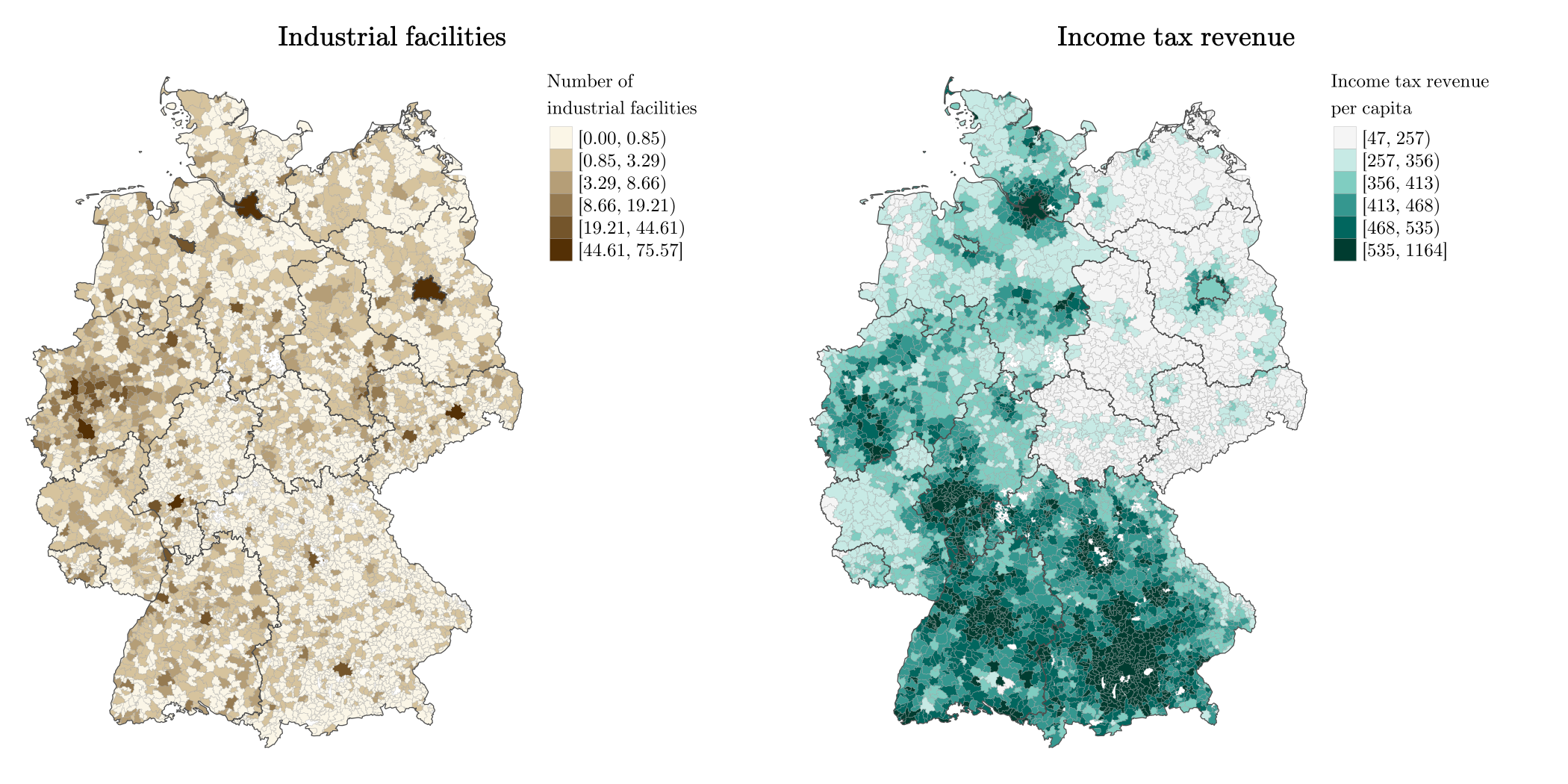
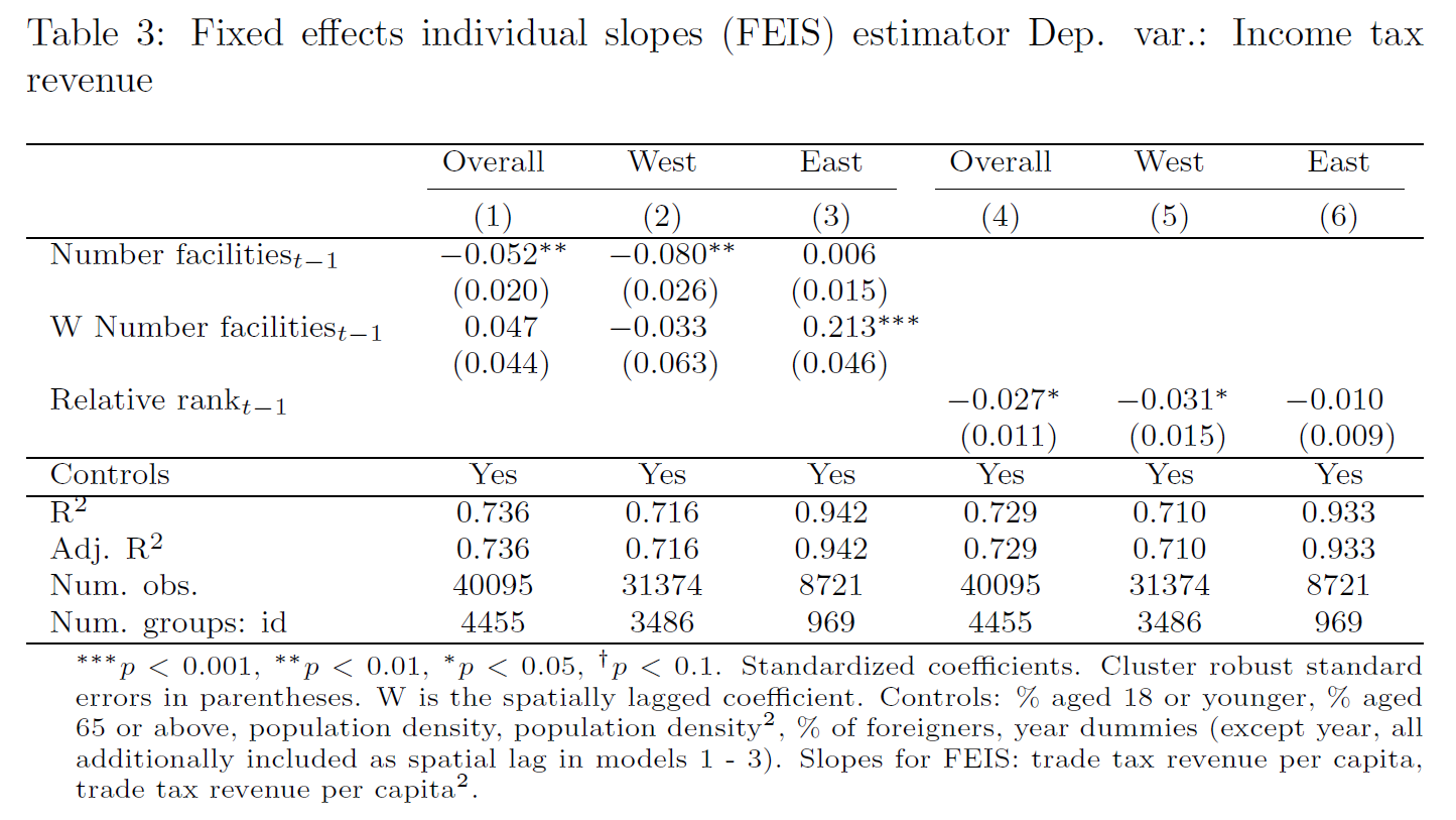
10.5 Example: Industrial facilities and municipal income

Rüttenauer and Best (2021): Environmental Inequality and Residential Sorting in Germany: A Spatial Time-Series Analysis of the Demographic Consequences of Industrial Sites. Demography, 58(6), 2243–2263. https://doi.org/10.1215/00703370-9563077

Spatial distribution of industrial facilities and income tax revenue per municipality for 2015.

Croissant, Yves, and Givanni Millo, eds. 2018. “Spatial Panels.” In Panel Data Econometrics with R, 245–84. Chichester, UK: John Wiley & Sons, Ltd. https://doi.org/10.1002/9781119504641.ch10.

Elhorst, J. Paul. 2012. “Dynamic Spatial Panels: Models, Methods, and Inferences.” Journal of Geographical Systems 14 (1): 5–28. https://doi.org/10.1007/s10109-011-0158-4.

———. 2014. Spatial Econometrics: From Cross-Sectional Data to Spatial Panels. SpringerBriefs in Regional Science. Berlin and Heidelberg: Springer. https://doi.org/10.1007/978-3-642-40340-8.

Fingleton, Bernard, Daniel Olner, and Gwilym Pryce. 2020. “Estimating the Local Employment Impacts of Immigration: A Dynamic Spatial Panel Model.” Urban Studies 57 (13): 2646–62. https://doi.org/10.1177/0042098019887916.

Lee, Lung-fei, and Jihai Yu. 2010. “Estimation of Spatial Autoregressive Panel Data Models with Fixed Effects.” Journal of Econometrics 154 (2): 165–85. https://doi.org/10.1016/j.jeconom.2009.08.001.

LeSage, James P. 2014. “Spatial Econometric Panel Data Model Specification: A Bayesian Approach.” Spatial Statistics 9 (August): 122–45. https://doi.org/10.1016/j.spasta.2014.02.002.

Millo, Giovanni, and Gianfranco Piras. 2012. “Splm: Spatial Panel Data Models in R.” Journal of Statistical Software 47 (1). https://doi.org/10.18637/jss.v047.i01.

Rüttenauer, Tobias, and Henning Best. 2021. “Environmental Inequality and Residential Sorting in Germany: A Spatial Time-Series Analysis of the Demographic Consequences of Industrial Sites.” Demography 58 (6): 2243–63. https://doi.org/10.1215/00703370-9563077.