Practical exercises: solutions
Tobias Rüttenauer
June 19, 2021
Required packages
pkgs <- c("sf", "mapview", "spdep", "spatialreg", "tmap", "tmaptools",
          "gstat", "randomForest", "nomisr") # note: load spdep first, then spatialreg
lapply(pkgs, require, character.only = TRUE)
Session info
sessionInfo()## R version 4.1.0 (2021-05-18)
## Platform: x86_64-w64-mingw32/x64 (64-bit)
## Running under: Windows 10 x64 (build 19042)
##
## Matrix products: default
##
## locale:
## [1] LC_COLLATE=English_United Kingdom.1252
## [2] LC_CTYPE=English_United Kingdom.1252
## [3] LC_MONETARY=English_United Kingdom.1252
## [4] LC_NUMERIC=C
## [5] LC_TIME=English_United Kingdom.1252
##
## attached base packages:
## [1] stats graphics grDevices utils datasets methods base
##
## other attached packages:
## [1] nomisr_0.4.4 randomForest_4.6-14 tmaptools_3.1-1
## [4] viridisLite_0.4.0 GWmodel_2.2-6 Rcpp_1.0.6
## [7] robustbase_0.93-8 maptools_1.1-1 tmap_3.3-1
## [10] spatialreg_1.1-8 Matrix_1.3-3 spdep_1.1-8
## [13] spData_0.3.8 sp_1.4-5 dplyr_1.0.6
## [16] rnaturalearth_0.1.0 nngeo_0.4.3 mapview_2.10.0
## [19] gstat_2.0-7 sf_1.0-0
##
## loaded via a namespace (and not attached):
## [1] leafem_0.1.6 colorspace_2.0-1 deldir_0.2-10
## [4] ellipsis_0.3.2 class_7.3-19 leaflet_2.0.4.1
## [7] rgdal_1.5-23 snakecase_0.11.0 satellite_1.0.2
## [10] base64enc_0.1-3 dichromat_2.0-0 proxy_0.4-26
## [13] farver_2.1.0 fansi_0.5.0 codetools_0.2-18
## [16] splines_4.1.0 knitr_1.33 jsonlite_1.7.2
## [19] png_0.1-7 rgeos_0.5-5 readr_1.4.0
## [22] compiler_4.1.0 httr_1.4.2 assertthat_0.2.1
## [25] s2_1.0.5 leaflet.providers_1.9.0 htmltools_0.5.1.1
## [28] tools_4.1.0 coda_0.19-4 glue_1.4.2
## [31] rnaturalearthdata_0.1.0 wk_0.4.1 gmodels_2.18.1
## [34] jquerylib_0.1.4 raster_3.4-10 vctrs_0.3.8
## [37] gdata_2.18.0 svglite_2.0.0 nlme_3.1-152
## [40] leafsync_0.1.0 crosstalk_1.1.1 lwgeom_0.2-6
## [43] xfun_0.23 stringr_1.4.0 lifecycle_1.0.0
## [46] gtools_3.9.2 XML_3.99-0.6 DEoptimR_1.0-9
## [49] LearnBayes_2.15.1 MASS_7.3-54 zoo_1.8-9
## [52] scales_1.1.1 rsdmx_0.6 hms_1.1.0
## [55] parallel_4.1.0 expm_0.999-6 RColorBrewer_1.1-2
## [58] yaml_2.2.1 sass_0.4.0 stringi_1.6.2
## [61] highr_0.9 leafpop_0.1.0 e1071_1.7-7
## [64] boot_1.3-28 intervals_0.15.2 rlang_0.4.11
## [67] pkgconfig_2.0.3 systemfonts_1.0.2 evaluate_0.14
## [70] lattice_0.20-44 purrr_0.3.4 htmlwidgets_1.5.3
## [73] tidyselect_1.1.1 plyr_1.8.6 magrittr_2.0.1
## [76] R6_2.5.0 generics_0.1.0 DBI_1.1.1
## [79] pillar_1.6.1 foreign_0.8-81 units_0.7-2
## [82] stars_0.5-3 xts_0.12.1 abind_1.4-5
## [85] tibble_3.1.2 spacetime_1.2-5 crayon_1.4.1
## [88] uuid_0.1-4 KernSmooth_2.23-20 utf8_1.2.1
## [91] rmarkdown_2.8 grid_4.1.0 FNN_1.1.3
## [94] digest_0.6.27 classInt_0.4-3 webshot_0.5.2
## [97] brew_1.0-6 stats4_4.1.0 munsell_0.5.0
## [100] bslib_0.2.5.1Load spatial data
See previous file.
load("_data/msoa_spatial.RData")Exercise 1
Add a control for the distance to Boris’ home (10 Downing St, London SW1A 2AB, UK).
* You could either find the coordinates manually or you use `tmaptools` function `geocode_OSM()` using OpenStreetMaps.

* There are also Google Maps APIs like `ggmap` or `mapsapi` but they require registration.
# Geocode an address using tmaptools
adr <- "10 Downing St, London SW1A 2AB, UK"
boris.spdf <- geocode_OSM(adr, as.sf = TRUE)
mapview(boris.spdf)# Transform into same projection
boris.spdf <- st_transform(boris.spdf, crs = st_crs(msoa.spdf))
# Copute distances betweens msoas and Boris
msoa.spdf$dist_boris <- st_distance(msoa.spdf, boris.spdf)
# Contiguity (Queens) neighbours weights
queens.nb <- poly2nb(msoa.spdf,
queen = TRUE,
snap = 1)
queens.lw <- nb2listw(queens.nb,
style = "W")
# Add to an SLX model (using queens.lw from previous script)
hv_2.slx <- lmSLX(log(Value) ~ log(POPDEN) + canopy_per + pubs_count + traffic + dist_boris,
data = msoa.spdf,
listw = queens.lw,
Durbin = as.formula( ~ log(POPDEN) + canopy_per +
pubs_count + traffic)) # we omit dist from the lagged vars
summary(hv_2.slx)##
## Call:
## lm(formula = formula(paste("y ~ ", paste(colnames(x)[-1], collapse = "+"))),
## data = as.data.frame(x), weights = weights)
##
## Residuals:
## Min 1Q Median 3Q Max
## -0.7461 -0.1810 -0.0376 0.1625 1.0780
##
## Coefficients:
## Estimate Std. Error t value Pr(>|t|)
## (Intercept) 1.393e+01 1.723e-01 80.810 < 2e-16 ***
## log.POPDEN. -1.027e-01 2.172e-02 -4.731 2.57e-06 ***
## canopy_per 5.965e-03 2.330e-03 2.560 0.01061 *
## pubs_count 1.744e-03 1.108e-03 1.573 0.11594
## traffic -8.218e-06 3.871e-06 -2.123 0.03401 *
## dist_boris -5.104e-05 3.269e-06 -15.616 < 2e-16 ***
## lag.log.POPDEN. -6.491e-02 3.497e-02 -1.856 0.06370 .
## lag.canopy_per 9.534e-03 3.055e-03 3.121 0.00186 **
## lag.pubs_count 8.224e-03 1.593e-03 5.162 2.97e-07 ***
## lag.traffic 1.259e-05 4.398e-06 2.862 0.00429 **
## ---
## Signif. codes: 0 '***' 0.001 '**' 0.01 '*' 0.05 '.' 0.1 ' ' 1
##
## Residual standard error: 0.2773 on 973 degrees of freedom
## Multiple R-squared: 0.4364, Adjusted R-squared: 0.4311
## F-statistic: 83.7 on 9 and 973 DF, p-value: < 2.2e-16Compared to previous results, adding the distance to Downing street, changed the effect of the lagged population density. So, our previous explanation based on centrality seems to make sense.
Exercise 2
How could we improve the interpolation of traffic counts based on idw()?
# Load traffic data
load("_data/traffic.RData")

# Set up regular grid over London with 1km cell size
london.sp <- st_union(st_geometry(msoa.spdf))
grid <- st_make_grid(london.sp, cellsize = 1000)
mapview(grid)
# Reduce to London bounds
grid <- grid[london.sp]
all_motor.idw <- idw(all_motor_vehicles ~ 1,
locations = traffic.spdf,
newdata = grid,
idp = 0.9, # Set decay lower
maxdist = 2000, # Define sharp cutoff
nmin = 5, # but use at least 5 points
force = TRUE) # even if there are less within maxdist## [inverse distance weighted interpolation]mapview(all_motor.idw[, "var1.pred"])Exercise 3
Can you think of a way of testing if higher order neighbours add additional information to the SLX regression model?
* The function `nblag()` is helpful.# Create neighbours of orders 1 to 3
queens.lag <- nblag(queens.nb, maxlag = 3)
# Create listwise of 1st, 2nd and 3rd order neighbours
queens.lw1 <- nb2listw(queens.lag[[1]], style = "W")
queens.lw2 <- nb2listw(queens.lag[[2]], style = "W")
queens.lw3 <- nb2listw(queens.lag[[3]], style = "W")
### Create lagged variables for different orders of neighbours
msoa.spdf$log_POPDEN <- log(msoa.spdf$POPDEN)
vars <- c("Value", "log_POPDEN", "canopy_per", "pubs_count", "traffic")
# lag1
w_vars <- create_WX(st_drop_geometry(msoa.spdf[, vars]),
listw = queens.lw1,
prefix = "w1")
msoa.spdf <- cbind(msoa.spdf, w_vars)
# lag2
w_vars <- create_WX(st_drop_geometry(msoa.spdf[, vars]),
listw = queens.lw2,
prefix = "w2")
msoa.spdf <- cbind(msoa.spdf, w_vars)
# lag3
w_vars <- create_WX(st_drop_geometry(msoa.spdf[, vars]),
listw = queens.lw3,
prefix = "w3")
msoa.spdf <- cbind(msoa.spdf, w_vars)
### LM to test imporatance
lm.mod <- lm(log(Value) ~ log_POPDEN + canopy_per + pubs_count + traffic +
w1.log_POPDEN + w1.canopy_per + w1.pubs_count + w1.traffic +
w2.log_POPDEN + w2.canopy_per + w2.pubs_count + w2.traffic +
w3.log_POPDEN + w3.canopy_per + w3.pubs_count + w3.traffic,
data = st_drop_geometry(msoa.spdf))
summary(lm.mod)##
## Call:
## lm(formula = log(Value) ~ log_POPDEN + canopy_per + pubs_count +
## traffic + w1.log_POPDEN + w1.canopy_per + w1.pubs_count +
## w1.traffic + w2.log_POPDEN + w2.canopy_per + w2.pubs_count +
## w2.traffic + w3.log_POPDEN + w3.canopy_per + w3.pubs_count +
## w3.traffic, data = st_drop_geometry(msoa.spdf))
##
## Residuals:
## Min 1Q Median 3Q Max
## -0.79853 -0.19413 -0.03608 0.16668 1.15518
##
## Coefficients:
## Estimate Std. Error t value Pr(>|t|)
## (Intercept) 1.142e+01 1.477e-01 77.344 < 2e-16 ***
## log_POPDEN -9.480e-02 2.283e-02 -4.152 3.59e-05 ***
## canopy_per 6.831e-03 2.544e-03 2.685 0.00738 **
## pubs_count 3.180e-03 1.158e-03 2.747 0.00613 **
## traffic -2.556e-06 4.702e-06 -0.544 0.58678
## w1.log_POPDEN 3.308e-02 4.243e-02 0.780 0.43583
## w1.canopy_per 5.057e-03 4.688e-03 1.079 0.28096
## w1.pubs_count 5.372e-03 2.024e-03 2.654 0.00809 **
## w1.traffic -2.770e-06 7.650e-06 -0.362 0.71730
## w2.log_POPDEN 7.559e-02 5.986e-02 1.263 0.20701
## w2.canopy_per 4.551e-03 5.561e-03 0.818 0.41328
## w2.pubs_count 3.883e-03 3.168e-03 1.226 0.22053
## w2.traffic 5.399e-06 6.678e-06 0.808 0.41901
## w3.log_POPDEN 2.543e-01 5.890e-02 4.317 1.74e-05 ***
## w3.canopy_per 6.903e-03 4.641e-03 1.487 0.13723
## w3.pubs_count 1.960e-02 3.233e-03 6.061 1.93e-09 ***
## w3.traffic -1.878e-06 4.350e-06 -0.432 0.66604
## ---
## Signif. codes: 0 '***' 0.001 '**' 0.01 '*' 0.05 '.' 0.1 ' ' 1
##
## Residual standard error: 0.2894 on 966 degrees of freedom
## Multiple R-squared: 0.3907, Adjusted R-squared: 0.3806
## F-statistic: 38.71 on 16 and 966 DF, p-value: < 2.2e-16### Random forest to test importance
# Train
rf.mod <- randomForest(log(Value) ~ log_POPDEN + canopy_per + pubs_count + traffic +
w1.log_POPDEN + w1.canopy_per + w1.pubs_count + w1.traffic +
w2.log_POPDEN + w2.canopy_per + w2.pubs_count + w2.traffic +
w3.log_POPDEN + w3.canopy_per + w3.pubs_count + w3.traffic,
data = st_drop_geometry(msoa.spdf),
mtry = 2,
ntree = 1000,
importance = TRUE)
# Inspect the mechanics of the model
importance(rf.mod)## %IncMSE IncNodePurity
## log_POPDEN 20.54317 5.619812
## canopy_per 25.63661 7.394993
## pubs_count 17.52750 5.289233
## traffic 21.56830 4.626584
## w1.log_POPDEN 22.83105 6.598008
## w1.canopy_per 30.78883 7.591774
## w1.pubs_count 31.73533 10.988702
## w1.traffic 24.68811 4.878405
## w2.log_POPDEN 23.41277 8.670035
## w2.canopy_per 26.22730 7.625017
## w2.pubs_count 31.43423 12.671079
## w2.traffic 30.38385 5.982058
## w3.log_POPDEN 23.73191 10.119258
## w3.canopy_per 28.61991 7.770954
## w3.pubs_count 31.10296 13.732942
## w3.traffic 33.80177 7.335586varImpPlot(rf.mod)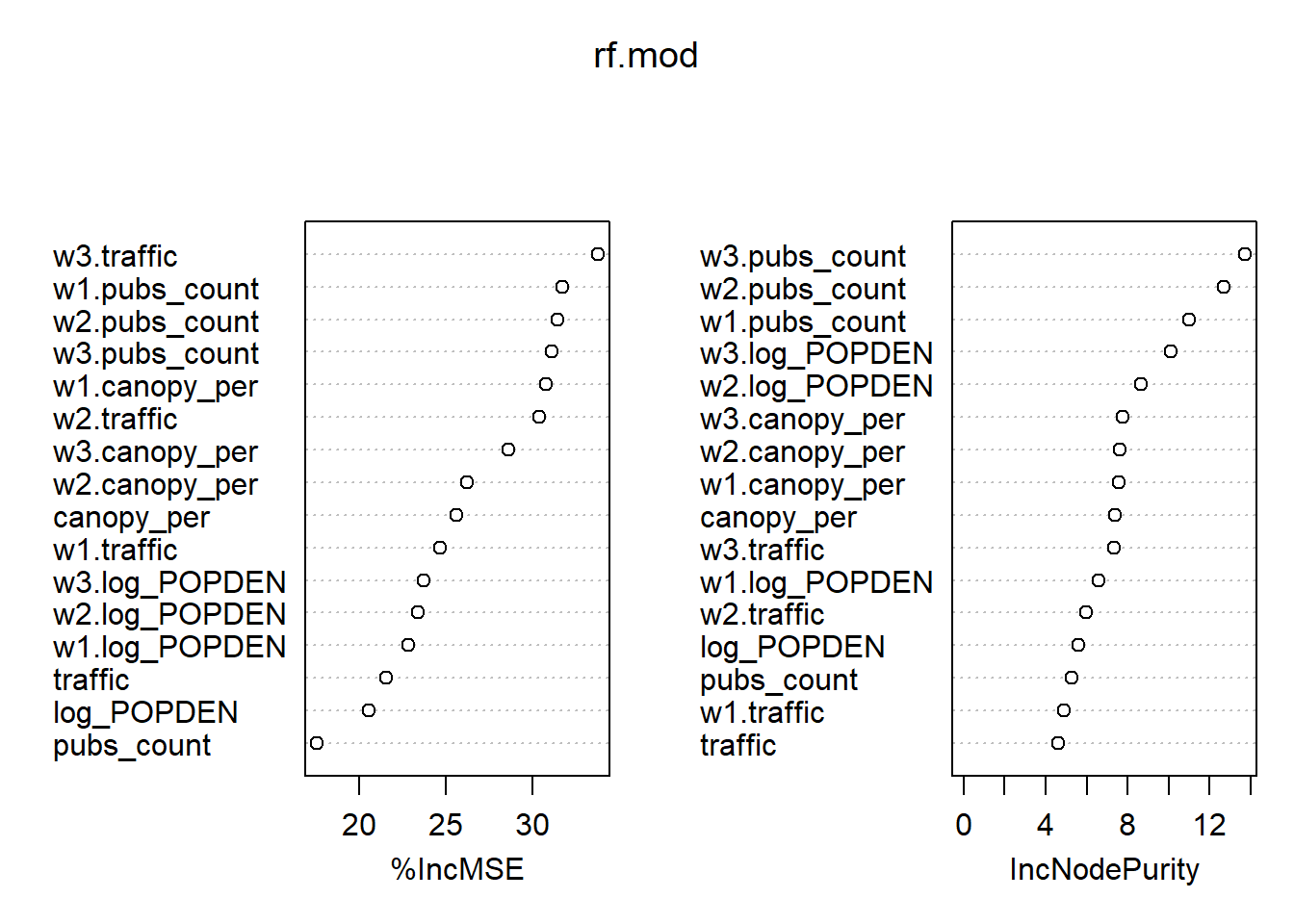
Exercise 4
Add the amount of particulate matter (PM10, e.g. 2017) from Defra and check if pollution influences the house values
* Note the following important sentence: "The coordinate system is OSGB and the coordinates represent the centre of each 1x1km cell".

* `st_buffer()` with the options `nQuadSegs  = 1, endCapStyle = 'SQUARE'` provides an easy way to get points into grids
# Download
pm10.link <- "https://uk-air.defra.gov.uk/datastore/pcm/mappm102017g.csv"
pm10.df <- read.csv(pm10.link, skip = 5, na.strings = "MISSING")
# Convert to sf point data
pm10.spdf <- st_as_sf(pm10.df,
coords = c("x", "y"), # Order is important
crs = 27700) # EPSG number of CRS
plot(pm10.spdf[1:100, "pm102017g"])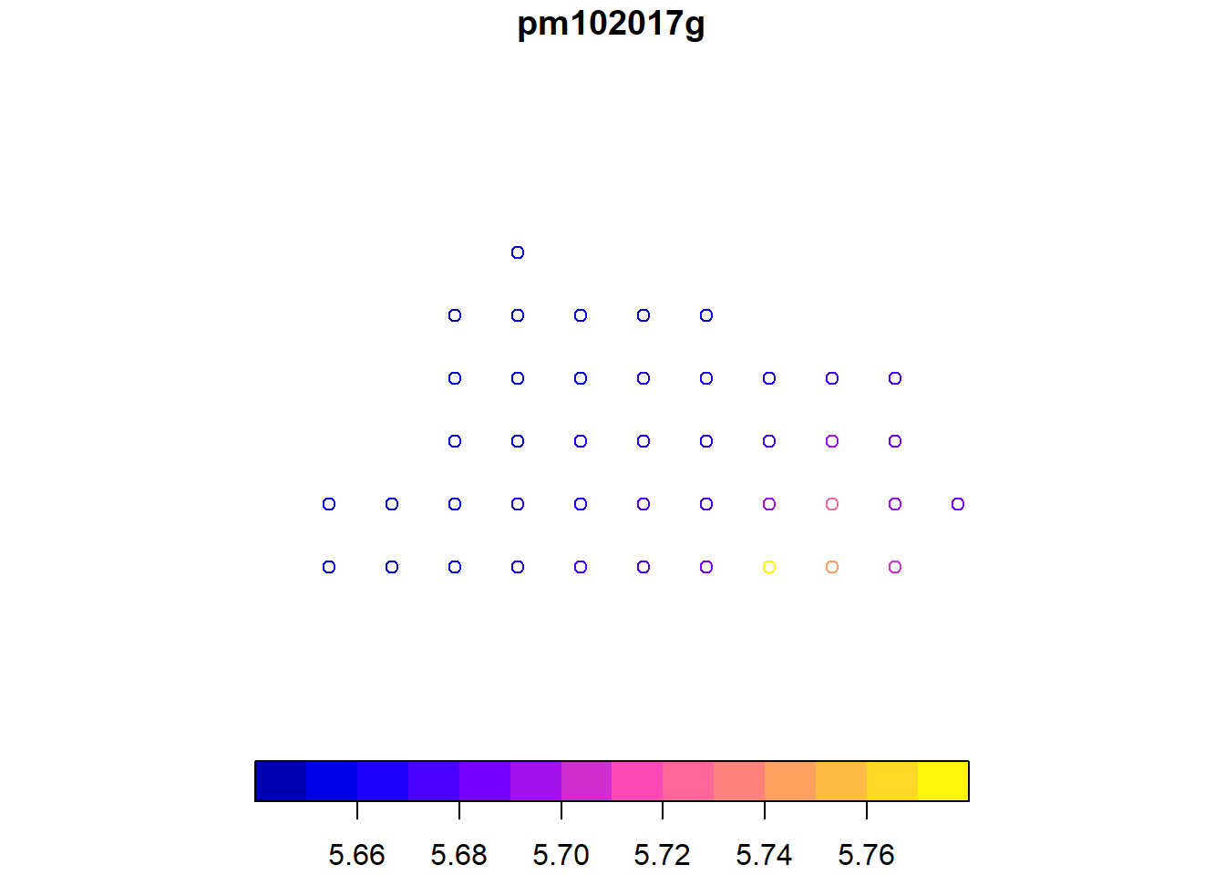
# Add qudratic buffer with 500m distance (1km/2) to get grid
pm10.spdf <- st_buffer(pm10.spdf, dist = 500, nQuadSegs  = 1,
                       endCapStyle = 'SQUARE')

plot(pm10.spdf[1:100, "pm102017g"])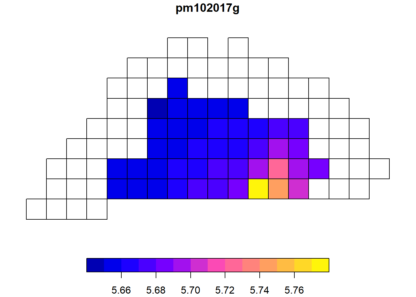
# Subset to London
pm10.spdf <- pm10.spdf[msoa.spdf, ]

plot(pm10.spdf[, "pm102017g"])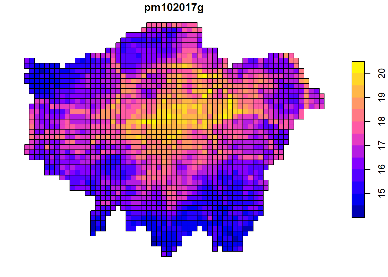
### Add to msoa data

# Calculate intersection
smoa_pm10.int <- st_intersection(msoa.spdf, pm10.spdf)
## Warning: attribute variables are assumed to be spatially constant throughout all
## geometries# average per MSOA
smoa_pm10.int <- aggregate(list(pm10 = smoa_pm10.int$pm102017g),
by = list(MSOA11CD = smoa_pm10.int$MSOA11CD),
mean)
# Merge back
msoa.spdf <- merge(msoa.spdf, smoa_pm10.int, by = "MSOA11CD", all.x = TRUE)
### Add to our SLX regression
hv_3.slx <- lmSLX(log(Value) ~ log(POPDEN) + canopy_per + pubs_count + traffic +
dist_boris + pm10,
data = msoa.spdf,
listw = queens.lw,
Durbin = as.formula( ~ log(POPDEN) + canopy_per +
pubs_count + traffic + pm10)) # we omit dist from the lagged vars
summary(hv_3.slx)##
## Call:
## lm(formula = formula(paste("y ~ ", paste(colnames(x)[-1], collapse = "+"))),
## data = as.data.frame(x), weights = weights)
##
## Residuals:
## Min 1Q Median 3Q Max
## -0.84301 -0.16841 -0.02519 0.14578 1.13275
##
## Coefficients:
## Estimate Std. Error t value Pr(>|t|)
## (Intercept) 1.554e+01 2.419e-01 64.264 < 2e-16 ***
## log.POPDEN. -7.076e-02 2.172e-02 -3.258 0.00116 **
## canopy_per 6.680e-03 2.267e-03 2.946 0.00330 **
## pubs_count 2.454e-03 1.066e-03 2.301 0.02157 *
## traffic -6.978e-06 3.920e-06 -1.780 0.07539 .
## dist_boris -5.792e-05 3.237e-06 -17.894 < 2e-16 ***
## pm10 -4.157e-02 4.106e-02 -1.012 0.31157
## lag.log.POPDEN. 1.184e-01 3.906e-02 3.032 0.00250 **
## lag.canopy_per 8.996e-03 2.948e-03 3.052 0.00234 **
## lag.pubs_count 1.207e-02 1.582e-03 7.628 5.67e-14 ***
## lag.traffic 1.855e-05 4.491e-06 4.131 3.92e-05 ***
## lag.pm10 -1.099e-01 4.447e-02 -2.471 0.01366 *
## ---
## Signif. codes: 0 '***' 0.001 '**' 0.01 '*' 0.05 '.' 0.1 ' ' 1
##
## Residual standard error: 0.2658 on 971 degrees of freedom
## Multiple R-squared: 0.4832, Adjusted R-squared: 0.4773
## F-statistic: 82.52 on 11 and 971 DF, p-value: < 2.2e-16Exercise 5
Add some more demographic variables from the Census 2011.
* The `nomisr` package provides an API to nomis. See the [Vignette](https://cran.r-project.org/web/packages/nomisr/vignettes/introduction.html). Make sure to restrict your request to London only (Guest users are limited to 25,000 rows per query).

* You can browse the available data online, such as the Census 2011 [key statistics](https://www.nomisweb.co.uk/census/2011/key_statistics_uk).
### For larger request, register and set key
# Sys.setenv(NOMIS_API_KEY = "XXX")
# nomis_api_key(check_env = TRUE)
x <- nomis_data_info()
# Get London ids
london_ids <- msoa.spdf$MSOA11CD
### Get key statistics ids
# select requires tables (https://www.nomisweb.co.uk/census/2011/key_statistics_uk)
# Get internal ids
stats <- c("KS401UK", "KS402UK")
oo <- which(grepl(paste(stats, collapse = "|"), x$name.value))
ksids <- x$id[oo]
ksids # This are the inernal ids## [1] "NM_1506_1" "NM_1507_1"### Lets look at meta information
q <- nomis_overview(ksids[1])
head(q)## # A tibble: 6 x 2
## name value
## <chr> <list>
## 1 analyses <named list [1]>
## 2 analysisname <chr [1]>
## 3 analysisnumber <int [1]>
## 4 contact <named list [4]>
## 5 contenttypes <named list [1]>
## 6 coverage <chr [1]>a <- nomis_get_metadata(id = ksids[1], concept = "GEOGRAPHY", type = "type")
a # TYPE297 is MSOA level## # A tibble: 17 x 3
## id label.en description.en
## <chr> <chr> <chr>
## 1 TYPE2~ 2011 scottish datazones 2011 scottish datazones
## 2 TYPE2~ 2011 scottish intermediate zones 2011 scottish intermediate zones
## 3 TYPE2~ 2011 census frozen wards 2011 census frozen wards
## 4 TYPE2~ 2011 NI small areas 2011 NI small areas
## 5 TYPE2~ Northern Ireland local governmen~ Northern Ireland local government d~
## 6 TYPE2~ 2011 scottish council areas 2011 scottish council areas
## 7 TYPE2~ 2011 super output areas - middle~ 2011 super output areas - middle la~
## 8 TYPE2~ 2011 super output areas - lower ~ 2011 super output areas - lower lay~
## 9 TYPE2~ 2011 output areas 2011 output areas
## 10 TYPE3~ 2001 scottish data zones 2001 scottish data zones
## 11 TYPE3~ 2001 northern ireland - super ou~ 2001 northern ireland - super outpu~
## 12 TYPE4~ local enterprise partnerships (a~ local enterprise partnerships (as o~
## 13 TYPE4~ parliamentary constituencies 2010 parliamentary constituencies 2010
## 14 TYPE4~ local authorities: county / unit~ local authorities: county / unitary~
## 15 TYPE4~ local authorities: district / un~ local authorities: district / unita~
## 16 TYPE4~ regions regions
## 17 TYPE4~ countries countriesb <- nomis_get_metadata(id = ksids[1], concept = "MEASURES", type = "TYPE297")
b # 20100 is the measure of absolute numbers## # A tibble: 2 x 3
## id label.en description.en
## <chr> <chr> <chr>
## 1 20100 value value
## 2 20301 percent percent### Query data in loop
for(i in ksids){
# Check if table is urban-rural devided
nd <- nomis_get_metadata(id = i)
if("RURAL_URBAN" %in% nd$conceptref){
UR <- TRUE
}else{
UR <- FALSE
}
# Query data
if(UR == TRUE){
ks_tmp <- nomis_get_data(id = i, time = "2011",
geography = london_ids, # replace with "TYPE297" for all
measures = 20100, RURAL_URBAN = 0)
}else{
ks_tmp <- nomis_get_data(id = i, time = "2011",
geography = london_ids, # replace with "TYPE297" for all
measures = 20100)
}
# Make lower case names
names(ks_tmp) <- tolower(names(ks_tmp))
names(ks_tmp)[names(ks_tmp) == "geography_code"] <- "msoa"
names(ks_tmp)[names(ks_tmp) == "geography_name"] <- "name"
# replace weird cell codes
onlynum <- which(grepl("^[[:digit:]]+$", ks_tmp$cell_code))
if(length(onlynum) != 0){
code <- substr(ks_tmp$cell_code[-onlynum][1], 1, 7)
ks_tmp$cell_code[onlynum] <- paste0(code, "_", ks_tmp$cell_code[onlynum])
}
# save codebook
ks_cb <- unique(ks_tmp[, c("date", "cell_type", "cell", "cell_code", "cell_name")])
### Reshape
ks_res <- tidyr::pivot_wider(ks_tmp, id_cols = c("msoa", "name"),
names_from = "cell_code",
values_from = "obs_value")
### Merge
if(i == ksids[1]){
census_keystat.df <- ks_res
census_keystat_cb.df <- ks_cb
}else{
census_keystat.df <- merge(census_keystat.df, ks_res, by = c("msoa", "name"), all = TRUE)
census_keystat_cb.df <- rbind(census_keystat_cb.df, ks_cb)
}
}##
## -- Column specification --------------------------------------------------------
## cols(
## .default = col_double(),
## DATE_TYPE = col_character(),
## GEOGRAPHY = col_character(),
## GEOGRAPHY_NAME = col_character(),
## GEOGRAPHY_CODE = col_character(),
## GEOGRAPHY_TYPE = col_character(),
## CELL_NAME = col_character(),
## CELL_CODE = col_character(),
## CELL_TYPE = col_character(),
## MEASURES_NAME = col_character(),
## OBS_STATUS = col_character(),
## OBS_STATUS_NAME = col_character(),
## OBS_CONF = col_logical(),
## OBS_CONF_NAME = col_character(),
## URN = col_character()
## )
## i Use `spec()` for the full column specifications.
##
##
## -- Column specification --------------------------------------------------------
## cols(
## .default = col_double(),
## DATE_TYPE = col_character(),
## GEOGRAPHY = col_character(),
## GEOGRAPHY_NAME = col_character(),
## GEOGRAPHY_CODE = col_character(),
## GEOGRAPHY_TYPE = col_character(),
## CELL_NAME = col_character(),
## CELL_CODE = col_character(),
## CELL_TYPE = col_character(),
## MEASURES_NAME = col_character(),
## OBS_STATUS = col_character(),
## OBS_STATUS_NAME = col_character(),
## OBS_CONF = col_logical(),
## OBS_CONF_NAME = col_character(),
## URN = col_character()
## )
## i Use `spec()` for the full column specifications.# Descirption are saved in the codebook
census_keystat_cb.df## # A tibble: 25 x 5
## date cell_type cell cell_code cell_name
## <dbl> <chr> <dbl> <chr> <chr>
## 1 2011 Dwelling Ty~ 0 KS401EW00~ All categories: Dwelling type
## 2 2011 Dwelling Ty~ 1 KS401EW00~ Unshared dwelling
## 3 2011 Dwelling Ty~ 2 KS401EW00~ Shared dwelling
## 4 2011 Dwelling Ty~ 3 KS401EW00~ All categories: Household spaces
## 5 2011 Dwelling Ty~ 4 KS401EW00~ Household spaces with at least one usual~
## 6 2011 Dwelling Ty~ 5 KS401EW00~ Household spaces with no usual residents
## 7 2011 Dwelling Ty~ 6 KS401EW00~ Whole house or bungalow: Detached
## 8 2011 Dwelling Ty~ 7 KS401EW00~ Whole house or bungalow: Semi-detached
## 9 2011 Dwelling Ty~ 8 KS401EW00~ Whole house or bungalow: Terraced (inclu~
## 10 2011 Dwelling Ty~ 9 KS401EW00~ Flat, maisonette or apartment: Purpose-b~
## # ... with 15 more rows### Merge with MSOA
msoa.spdf <- merge(msoa.spdf, census_keystat.df,
by.x = "MSOA11CD", by.y = "msoa", all.x = TRUE)