Part 1: Using and linking spatial data
Tobias Rüttenauer
June 19, 2021
Required packages
pkgs <- c("sf", "gstat", "mapview", "nngeo", "rnaturalearth", "dplyr")
lapply(pkgs, require, character.only = TRUE)Session info
sessionInfo()## R version 4.1.0 (2021-05-18)
## Platform: x86_64-w64-mingw32/x64 (64-bit)
## Running under: Windows 10 x64 (build 19042)
##
## Matrix products: default
##
## locale:
## [1] LC_COLLATE=English_United Kingdom.1252
## [2] LC_CTYPE=English_United Kingdom.1252
## [3] LC_MONETARY=English_United Kingdom.1252
## [4] LC_NUMERIC=C
## [5] LC_TIME=English_United Kingdom.1252
##
## attached base packages:
## [1] stats graphics grDevices utils datasets methods base
##
## other attached packages:
## [1] dplyr_1.0.6 rnaturalearth_0.1.0 nngeo_0.4.3
## [4] mapview_2.10.0 gstat_2.0-7 sf_1.0-0
##
## loaded via a namespace (and not attached):
## [1] zoo_1.8-9 tidyselect_1.1.1 xfun_0.23 bslib_0.2.5.1
## [5] purrr_0.3.4 lattice_0.20-44 colorspace_2.0-1 vctrs_0.3.8
## [9] generics_0.1.0 stats4_4.1.0 htmltools_0.5.1.1 spacetime_1.2-5
## [13] yaml_2.2.1 base64enc_0.1-3 utf8_1.2.1 rlang_0.4.11
## [17] e1071_1.7-7 jquerylib_0.1.4 pillar_1.6.1 glue_1.4.2
## [21] DBI_1.1.1 sp_1.4-5 lifecycle_1.0.0 stringr_1.4.0
## [25] munsell_0.5.0 raster_3.4-10 htmlwidgets_1.5.3 codetools_0.2-18
## [29] evaluate_0.14 knitr_1.33 crosstalk_1.1.1 class_7.3-19
## [33] fansi_0.5.0 leafem_0.1.6 xts_0.12.1 Rcpp_1.0.6
## [37] KernSmooth_2.23-20 scales_1.1.1 satellite_1.0.2 classInt_0.4-3
## [41] webshot_0.5.2 leaflet_2.0.4.1 jsonlite_1.7.2 FNN_1.1.3
## [45] png_0.1-7 digest_0.6.27 stringi_1.6.2 grid_4.1.0
## [49] tools_4.1.0 magrittr_2.0.1 sass_0.4.0 proxy_0.4-26
## [53] tibble_3.1.2 crayon_1.4.1 pkgconfig_2.0.3 ellipsis_0.3.2
## [57] assertthat_0.2.1 rmarkdown_2.8 R6_2.5.0 units_0.7-2
## [61] intervals_0.15.2 compiler_4.1.0Coordinates
In general, spatial data is structured like conventional data (e.g. data.frames, matrices), but has one additional dimension: every observation is linked to some sort of geo-spatial information. Most common types of spatial information are:
Points (one coordinate pair)
Lines (two coordinate pairs)
Polygons (at least three coordinate pairs)
Regular grids (one coordinate pair for centroid + raster / grid size)
Coordinate reference system (CRS)
In its raw form, a pair of coordinates consists of two numerical values. For instance, the pair c(51.752595, -1.262801) describes the location of Nuffield College in Oxford (one point). The fist number represents the latitude (north-south direction), the second number is the longitude (west-east direction), both are in decimal degrees.
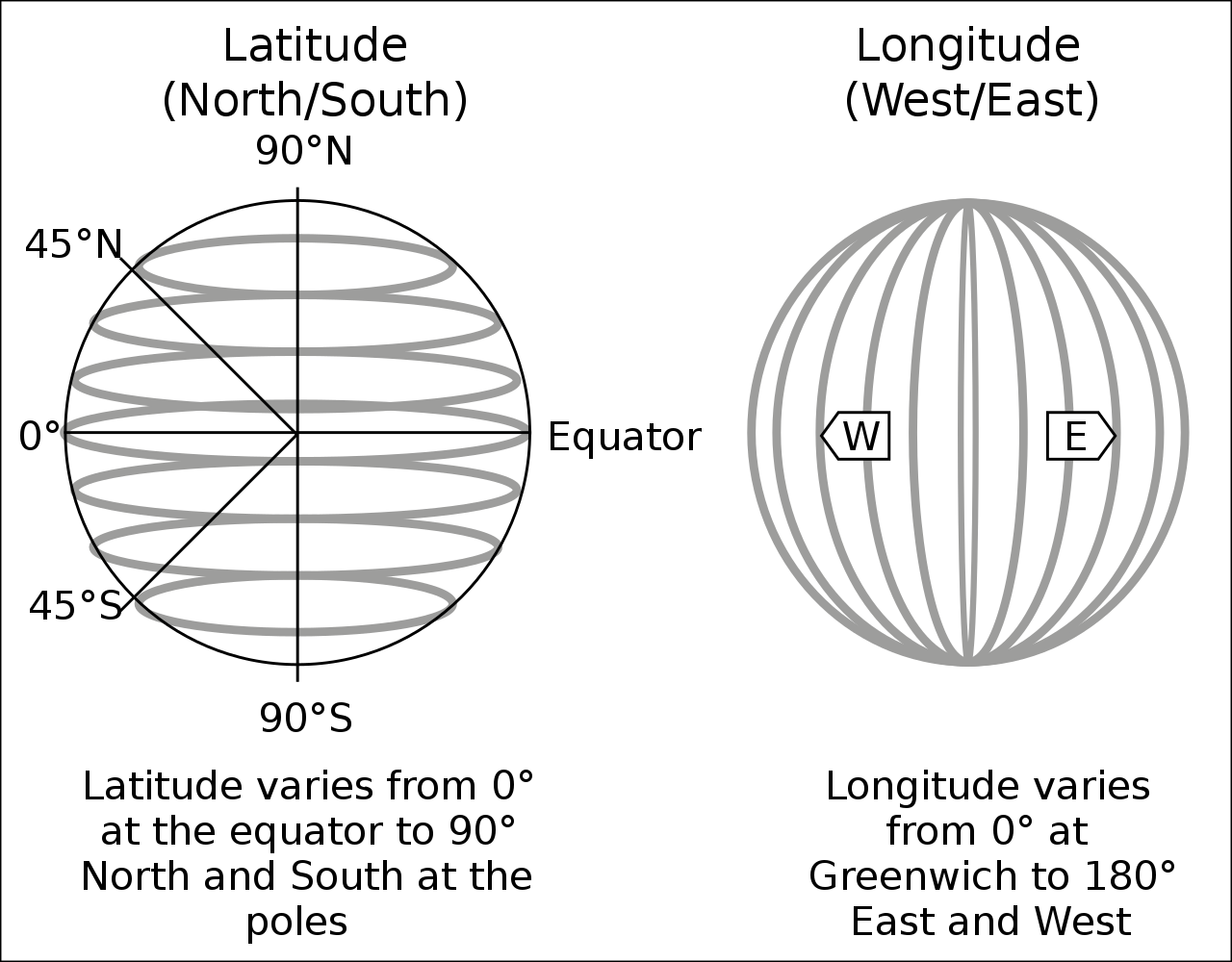
Figure: Latitude and longitude, Source: Wikipedia
However, we need to specify a reference point for latitudes and longitudes (in the Figure above: equator and Greenwich). For instance, the pair of coordinates above comes from the Google Maps, which returns GPS coordinates in ‘WGS 84’ (EPSG:4326).
# Coordinate pairs of two locations
coords1 <- c(51.752595, -1.262801)
coords2 <- c(51.753237, -1.253904)
coords <- rbind(coords1, coords2)
# Conventional data frame
nuffield.df <- data.frame(name = c("Nuffield College", "Radcliffe Camera"),
address = c("New Road", "Radcliffe Sq"),
lat = coords[,1], lon = coords[,2])
head(nuffield.df)## name address lat lon
## coords1 Nuffield College New Road 51.75259 -1.262801
## coords2 Radcliffe Camera Radcliffe Sq 51.75324 -1.253904# Combine to spatial data frame
nuffield.spdf <- st_as_sf(nuffield.df,
coords = c("lon", "lat"), # Order is important
crs = 4326) # EPSG number of CRS
# Map
mapview(nuffield.spdf, zcol = "name")Projected CRS
However, different data providers use different CRS. For instance, spatial data in the UK usually uses ‘OSGB 1936 / British National Grid’ (EPSG:27700). Here, coordinates are in meters, and projected onto a planar 2D space.
There are a lot of different CRS projections, and different national statistics offices provide data in different projections. Data providers usually specify which reference system they use. This is important as using the correct reference system and projection is crucial for plotting and manipulating spatial data.
If you do not know the correct CRS, try starting with a standards CRS like EPSG:4326 if you have decimal degree like coordinates. If it looks like projected coordinates, try searching for the country or region in CRS libraries like https://epsg.io/. However, you must check if the projected coordinates match their real location, e.g. using mpaview().
Why different projections?
By now, (most) people agree that the earth is not flat. So, to plot data on a 2D planar surface and to perform certain operations on a planar world, we need to make some re-projections. Depending on where we are, different re-projections of our data might work better than others.
world <- ne_countries(scale = "medium", returnclass = "sf")
class(world)## [1] "sf" "data.frame"st_crs(world)## Coordinate Reference System:
## User input: +proj=longlat +datum=WGS84 +no_defs +ellps=WGS84 +towgs84=0,0,0
## wkt:
## BOUNDCRS[
## SOURCECRS[
## GEOGCRS["unknown",
## DATUM["World Geodetic System 1984",
## ELLIPSOID["WGS 84",6378137,298.257223563,
## LENGTHUNIT["metre",1]],
## ID["EPSG",6326]],
## PRIMEM["Greenwich",0,
## ANGLEUNIT["degree",0.0174532925199433],
## ID["EPSG",8901]],
## CS[ellipsoidal,2],
## AXIS["longitude",east,
## ORDER[1],
## ANGLEUNIT["degree",0.0174532925199433,
## ID["EPSG",9122]]],
## AXIS["latitude",north,
## ORDER[2],
## ANGLEUNIT["degree",0.0174532925199433,
## ID["EPSG",9122]]]]],
## TARGETCRS[
## GEOGCRS["WGS 84",
## DATUM["World Geodetic System 1984",
## ELLIPSOID["WGS 84",6378137,298.257223563,
## LENGTHUNIT["metre",1]]],
## PRIMEM["Greenwich",0,
## ANGLEUNIT["degree",0.0174532925199433]],
## CS[ellipsoidal,2],
## AXIS["latitude",north,
## ORDER[1],
## ANGLEUNIT["degree",0.0174532925199433]],
## AXIS["longitude",east,
## ORDER[2],
## ANGLEUNIT["degree",0.0174532925199433]],
## ID["EPSG",4326]]],
## ABRIDGEDTRANSFORMATION["Transformation from unknown to WGS84",
## METHOD["Geocentric translations (geog2D domain)",
## ID["EPSG",9603]],
## PARAMETER["X-axis translation",0,
## ID["EPSG",8605]],
## PARAMETER["Y-axis translation",0,
## ID["EPSG",8606]],
## PARAMETER["Z-axis translation",0,
## ID["EPSG",8607]]]]# Extract a country and plot in current CRS (WGS84)
ger.spdf <- world[world$name == "Germany", ]
plot(st_geometry(ger.spdf))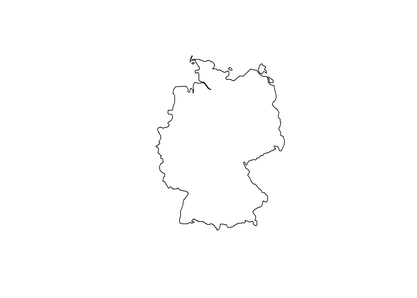
# Now, lets transform Germany into a CRS optimized for Iceland
ger_rep.spdf <- st_transform(ger.spdf, crs = 5325)
plot(st_geometry(ger_rep.spdf))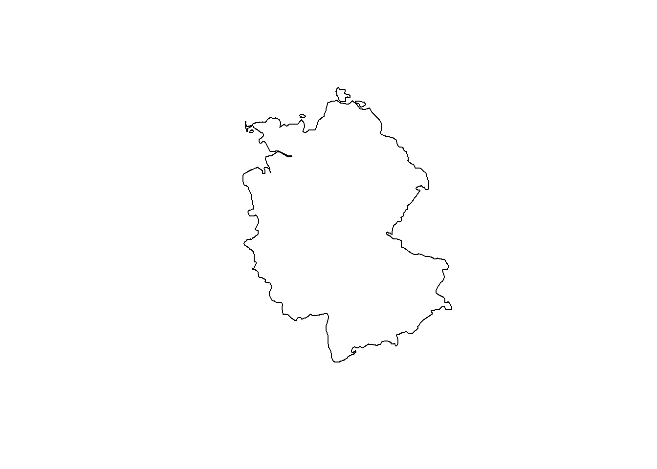
Depending on the angle, a 2D projection of the earth looks different. It is important to choose a suitable projection for the available spatial data. For more information on CRS and re-projection, see e.g. Lovelace, Nowosad, and Muenchow (2019).
Importing some real word data
sf imports many of the most common spatial data files, like geojson, gpkg, or shp.
London shapefile (polygon)
Lets get some administrative boundaries for London from the London Datastore.
# Create subdir
dn <- "_data"
ifelse(dir.exists(dn), "Exists", dir.create(dn))## [1] "Exists"# Download zip file and unzip
tmpf <- tempfile()
boundary.link <- "https://data.london.gov.uk/download/statistical-gis-boundary-files-london/9ba8c833-6370-4b11-abdc-314aa020d5e0/statistical-gis-boundaries-london.zip"
download.file(boundary.link, tmpf)
unzip(zipfile = tmpf, exdir = paste0(dn))
unlink(tmpf)
# We only need the MSOA layer for now
msoa.spdf <- st_read(dsn = paste0(dn, "/statistical-gis-boundaries-london/ESRI"),
layer = "MSOA_2011_London_gen_MHW" # Note: no file ending
)## Reading layer `MSOA_2011_London_gen_MHW' from data source
## `C:\work\Lehre\SICSS_Spatial\_data\statistical-gis-boundaries-london\ESRI'
## using driver `ESRI Shapefile'
## Simple feature collection with 983 features and 12 fields
## Geometry type: MULTIPOLYGON
## Dimension: XY
## Bounding box: xmin: 503574.2 ymin: 155850.8 xmax: 561956.7 ymax: 200933.6
## Projected CRS: OSGB 1936 / British National Gridhead(msoa.spdf)## Simple feature collection with 6 features and 12 fields
## Geometry type: MULTIPOLYGON
## Dimension: XY
## Bounding box: xmin: 530966.7 ymin: 180510.7 xmax: 551943.8 ymax: 191139
## Projected CRS: OSGB 1936 / British National Grid
## MSOA11CD MSOA11NM LAD11CD LAD11NM RGN11CD
## 1 E02000001 City of London 001 E09000001 City of London E12000007
## 2 E02000002 Barking and Dagenham 001 E09000002 Barking and Dagenham E12000007
## 3 E02000003 Barking and Dagenham 002 E09000002 Barking and Dagenham E12000007
## 4 E02000004 Barking and Dagenham 003 E09000002 Barking and Dagenham E12000007
## 5 E02000005 Barking and Dagenham 004 E09000002 Barking and Dagenham E12000007
## 6 E02000007 Barking and Dagenham 006 E09000002 Barking and Dagenham E12000007
## RGN11NM USUALRES HHOLDRES COMESTRES POPDEN HHOLDS AVHHOLDSZ
## 1 London 7375 7187 188 25.5 4385 1.6
## 2 London 6775 6724 51 31.3 2713 2.5
## 3 London 10045 10033 12 46.9 3834 2.6
## 4 London 6182 5937 245 24.8 2318 2.6
## 5 London 8562 8562 0 72.1 3183 2.7
## 6 London 8791 8672 119 50.6 3441 2.5
## geometry
## 1 MULTIPOLYGON (((531667.6 18...
## 2 MULTIPOLYGON (((548881.6 19...
## 3 MULTIPOLYGON (((549102.4 18...
## 4 MULTIPOLYGON (((551550 1873...
## 5 MULTIPOLYGON (((549099.6 18...
## 6 MULTIPOLYGON (((549819.9 18...This looks like a conventional data.frame but has the additional column geometry containing the coordinates of each observation. st_geometry() returns only the geographic object and st_drop_geometry() only the data.frame without the coordinates. We can plot the object using mapview().
mapview(msoa.spdf[, "POPDEN"])And we add the median house prices in 2017 from the London Datastore.
# Download
hp.link <- "https://data.london.gov.uk/download/average-house-prices/bdf8eee7-41e1-4d24-90ce-93fe5cf040ae/land-registry-house-prices-MSOA.csv"
hp.df <- read.csv(hp.link)
hp.df <- hp.df[which(hp.df$Measure == "Median" &
hp.df$Year == "Year ending Sep 2017"), ]
hp.df$Value <- as.numeric(hp.df$Value)
# Merge (as with conventional df)
msoa.spdf <- merge(msoa.spdf, hp.df,
by.x = "MSOA11CD", by.y = "Code",
all.x = TRUE, all.y = FALSE)
mapview(msoa.spdf[, "Value"])Tree cover (gridded)
The London Tree Canopy Cover data provides data on tree coverage in London based on high-resolution imagery and machine learning techniques, again available at London Datastore.
# Download zip shapefile
tmpf <- tempfile()
trees.link <- "https://data.london.gov.uk/download/curio-canopy/4fd54ef7-195f-43dc-a0d1-24e96e876f6c/shp-hexagon-files.zip"
download.file(trees.link, tmpf)
unzip(zipfile = tmpf, exdir = paste0(dn))
unlink(tmpf)
trees.spdf <- st_read(dsn = paste0(dn, "/shp-hexagon-files"),
layer = "gla-canopy-hex")## Reading layer `gla-canopy-hex' from data source
## `C:\work\Lehre\SICSS_Spatial\_data\shp-hexagon-files' using driver `ESRI Shapefile'
## Simple feature collection with 15041 features and 6 fields
## Geometry type: POLYGON
## Dimension: XY
## Bounding box: xmin: 503669.2 ymin: 155850.8 xmax: 561967.2 ymax: 201000.8
## Projected CRS: OSGB 1936 / British National Gridmapview(trees.spdf[, "canopy_per"])Cultural venues (point)
Environmental features might be important for housing prices, but - obviously - what counts are the number of proximate pubs? So, lets get some info on cultural venues, again from London Datastore.
culture.link <- "https://data.london.gov.uk/download/cultural-infrastructure-map/bf7822ed-e90a-4773-abef-dda6f6b40654/CulturalInfrastructureMap.gpkg"
# This time, we have Geopackage format (gpkg)
tmpf <- tempfile(fileext = ".gpkg")
download.file(culture.link, destfile = tmpf, mode = "wb")
# And we only load the layer containing pubs
st_layers(tmpf)## Driver: GPKG
## Available layers:
## layer_name geometry_type features fields
## 1 Set_and_exhibition_building Point 46 15
## 2 Skate_Parks Point 50 15
## 3 Textile_design Point 81 15
## 4 Theatre_rehearsal_studio Point 118 15
## 5 Theatres Point 264 15
## 6 Archives Point 557 15
## 7 Artists_workspaces Point 240 15
## 8 Arts_centres Point 26 15
## 9 Cinemas Point 116 15
## 10 Commercial_galleries Point 306 15
## 11 Community_centres Point 903 18
## 12 Creative_coworking_desk_space Point 50 15
## 13 Creative_workspaces Point 84 15
## 14 Dance_performance_venues Point 190 15
## 15 Dance_rehearsal_studios Point 265 15
## 16 Fashion_and_design Point 159 15
## 17 Heritage_at_risk Point 746 15
## 18 Jewellery_design Point 320 15
## 19 Large_media_production_studios Point 5 19
## 20 Legal_street_art_walls Point 6 15
## 21 LGBT_night_time_venues Point 75 15
## 22 Libraries Point 342 15
## 23 Listed_buildings Point 19243 14
## 24 Live_in_artists_workspace Point 8 15
## 25 Makerspaces Point 74 15
## 26 Making_and_manufacturing Point 43 15
## 27 Museums_and_public_galleries Point 163 15
## 28 Music_office_based_businesses Point 304 15
## 29 Music_recording_studios Point 71 15
## 30 Music_rehearsal_studios Point 79 15
## 31 Music_venues_all Point 797 15
## 32 Music_venues_grassroots Point 100 15
## 33 Outdoor_spaces_for_cultural_use Point 17 17
## 34 Prop_and_costume_making Point 55 15
## 35 Pubs Point 4098 15pubs.spdf <- st_read(dsn = tmpf, layer = "Pubs")## Reading layer `Pubs' from data source
## `C:\Users\tobias.ruettenauer\AppData\Local\Temp\RtmpcpkjG3\file14e410ed6eb6.gpkg'
## using driver `GPKG'
## Simple feature collection with 4098 features and 15 fields
## Geometry type: POINT
## Dimension: XY
## Bounding box: xmin: 504622 ymin: 156900.9 xmax: 559327 ymax: 199982.9
## Projected CRS: OSGB 1936 / British National Gridunlink(tmpf)
mapview(st_geometry(pubs.spdf))Manipulation and linkage
Having data with geo-spatial information allows to perform a variety of methods to manipulate and link different data sources. Commonly used methods include 1) subsetting, 2) point-in-polygon operations, 3) distance measures, 4) intersections or buffer methods.
The online Vignettes of the sf package provide a comprehensive overview of the multiple ways of spatial manipulations.
Check if data is on common projection
st_crs(msoa.spdf) == st_crs(trees.spdf)## [1] FALSEst_crs(trees.spdf) == st_crs(pubs.spdf)## [1] TRUE# MSOA in different crs --> transform
msoa.spdf <- st_transform(msoa.spdf, crs = st_crs(trees.spdf))
# Check if all geometries are valid, and make valid if needed
msoa.spdf <- st_make_valid(msoa.spdf)Subsetting
We can subset spatial data in a similar way as we subset conventional data.frame or matrices. For instance, lets find all pubs in Westminster.
# Subset msoa and combine to one unit
westminster.spdf <- msoa.spdf[msoa.spdf$LAD11NM == "Westminster",]
westminster.spdf <- st_union(westminster.spdf)
# Subset to points in this area
sub1.spdf <- pubs.spdf[westminster.spdf, ] # or:
sub1.spdf <- st_filter(pubs.spdf, westminster.spdf)
mapview(sub1.spdf)Or we can reverse the above and exclude all intersecting pubs by specifying st_disjoint as alternative spatial operation using the op = option (note the empty space for column selection). st_filter() with the .predicate option does the same job. See the sf Vignette for more operations.
# Subset to points not in this area
sub2.spdf <- pubs.spdf[westminster.spdf, , op = st_disjoint] # or:
sub2.spdf <- st_filter(pubs.spdf, westminster.spdf, .predicate = st_disjoint)
mapview(list(sub1.spdf, sub2.spdf), col.regions = list("red", "blue"))Point in polygon
We are interested in the number of pubs in each MSOA. So, we count the number of points in each polygon.
# Assign MSOA to each point
pubs_msoa.join <- st_join(pubs.spdf, msoa.spdf, join = st_within)
# Count N by MSOA code (drop geometry to speed up)
pubs_msoa.join <- dplyr::count(st_drop_geometry(pubs_msoa.join),
MSOA11CD = pubs_msoa.join$MSOA11CD,
name = "pubs_count")
sum(pubs_msoa.join$pubs_count)## [1] 4098# Merge and replace NAs with zero (no matches, no pubs)
msoa.spdf <- merge(msoa.spdf, pubs_msoa.join,
by = "MSOA11CD", all.x = TRUE)
msoa.spdf$pubs_count[is.na(msoa.spdf$pubs_count)] <- 0Distance measures
We might be interested in the distance to the nearest forest / green area. Here, we use the package nngeo to find k nearest neighbours with the respective distance.
hist(trees.spdf$canopy_per)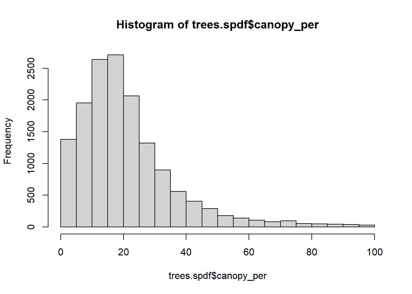
# Select areas with at least 50% tree coverage
trees_high.spdf <- trees.spdf[trees.spdf$canopy_per >= 50, ]
mapview(trees_high.spdf[, "canopy_per"])# Use geometric centroid of each MSOA
cent.sp <- st_centroid(msoa.spdf[, "MSOA11CD"])## Warning in st_centroid.sf(msoa.spdf[, "MSOA11CD"]): st_centroid assumes
## attributes are constant over geometries of x# Get K nearest neighbour with distance
knb.dist <- st_nn(cent.sp, trees_high.spdf,
k = 1, returnDist = TRUE,
progress = FALSE)## lines or polygonsmsoa.spdf$dist_trees50 <- unlist(knb.dist$dist)
summary(msoa.spdf$dist_trees50)## Min. 1st Qu. Median Mean 3rd Qu. Max.
## 0 740 1340 1515 2096 4858Intersections + Buffers
We might also be interested in the average tree cover density within 1 km radius around each MSOA centroid. Therefore, we first create a buffer with st_buffer() around each midpoint and subsequently use st_intersetion() to calculate the overlap.
# Create buffer (1km radius)
cent.buf <- st_buffer(cent.sp, dist = 1000)
mapview(cent.buf)# Calculate intersection between buffers and tree-cover hexagons
buf_hex.int <- st_intersection(cent.buf, trees.spdf)## Warning: attribute variables are assumed to be spatially constant throughout all
## geometriesdim(buf_hex.int)## [1] 41100 8# We could also calculate the area of overlap for each pair (to calculate weighted averages)
buf_hex.int$area <- as.numeric(st_area(buf_hex.int))
# Or we just use the simple average per each MSOA
buf_hex.int <- aggregate(list(canopy_per = buf_hex.int$canopy_per),
by = list(MSOA11CD = buf_hex.int$MSOA11CD),
mean)
# Merge back to spatial data.frame
msoa.spdf <- merge(msoa.spdf, buf_hex.int, by = "MSOA11CD", all.x = TRUE)Note: for buffer related methods, it often makes sense to use population weighted centroids instead of geographic centroids (see here for MSOA population weighted centroids). However, often this information is not available.
Interpolation and Kriging
For (sparse) point data, we the nearest count point often might be far away from where we want to measure or merge its attributes. A potential solution is to spatially interpolate the data (e.g. on a regular grid): given a specific function of space (and covariates), we make prediction about an attribute at “missing” locations. For more details, see, for instance, Spatial Data Science or Introduction to Spatial Data Programming with R.
First lets get some point data with associated attributes or measures. In this example, we use traffic counts provided by the Department for Transport.
# Download
traffic.link <- "https://dft-statistics.s3.amazonaws.com/road-traffic/downloads/aadf/region_id/dft_aadf_region_id_6.csv"
traffic.df <- read.csv(traffic.link)
traffic.df <- traffic.df[which(traffic.df$year == 2017 &
traffic.df$road_type == "Major"), ]
names(traffic.df)## [1] "count_point_id" "year"
## [3] "region_id" "region_name"
## [5] "local_authority_id" "local_authority_name"
## [7] "road_name" "road_type"
## [9] "start_junction_road_name" "end_junction_road_name"
## [11] "easting" "northing"
## [13] "latitude" "longitude"
## [15] "link_length_km" "link_length_miles"
## [17] "estimation_method" "estimation_method_detailed"
## [19] "pedal_cycles" "two_wheeled_motor_vehicles"
## [21] "cars_and_taxis" "buses_and_coaches"
## [23] "lgvs" "hgvs_2_rigid_axle"
## [25] "hgvs_3_rigid_axle" "hgvs_4_or_more_rigid_axle"
## [27] "hgvs_3_or_4_articulated_axle" "hgvs_5_articulated_axle"
## [29] "hgvs_6_articulated_axle" "all_hgvs"
## [31] "all_motor_vehicles"# Transform to spatial data
traffic.spdf <- st_as_sf(traffic.df,
coords = c("longitude", "latitude"),
crs = 4326)
# Transform into common crs
traffic.spdf <- st_transform(traffic.spdf,
crs = st_crs(msoa.spdf))
# Map
mapview(traffic.spdf[, "all_motor_vehicles"])# Save (for later exercise)
save(traffic.spdf, file = "_data/traffic.RData")To interpolate, we first create a grid surface over London on which we make predictions.
# Set up regular grid over London with 1km cell size
london.sp <- st_union(st_geometry(msoa.spdf))
grid <- st_make_grid(london.sp, cellsize = 1000)
mapview(grid)# Reduce to London bounds
grid <- grid[london.sp]
mapview(grid)There are various ways of interpolating. Common methods are nearest neighbours matching or inverse distance weighted interpolation (using idw()): each value at a given point is a weighted average of surrounding values, where weights are a function of distance.
# IDW interpolation
all_motor.idw <- idw(all_motor_vehicles ~ 1,
locations = traffic.spdf,
newdata = grid,
idp = 2) # power of distance decay## [inverse distance weighted interpolation]mapview(all_motor.idw[, "var1.pred"])IDW is a fairly simple way of interpolation and it assumes a deterministic form of spatial dependence.
Another technique is Kriging, which estimates values as a function of a deterministic trend and a random process. However, we have to set some hyper-parameters for that: sill, range, nugget, and the functional form. Therefore, we first need to fit a semi-variogram. Subsequently, we let the fit.variogram() function chose the parameters based on the empirical variogram [see for instance r-spatial Homepage].
# Variogram
all_motor.var <- variogram(all_motor_vehicles ~ 1,
traffic.spdf)## Warning in showSRID(SRS_string, format = "PROJ", multiline = "NO", prefer_proj =
## prefer_proj): Discarded datum OSGB 1936 in Proj4 definitionplot(all_motor.var)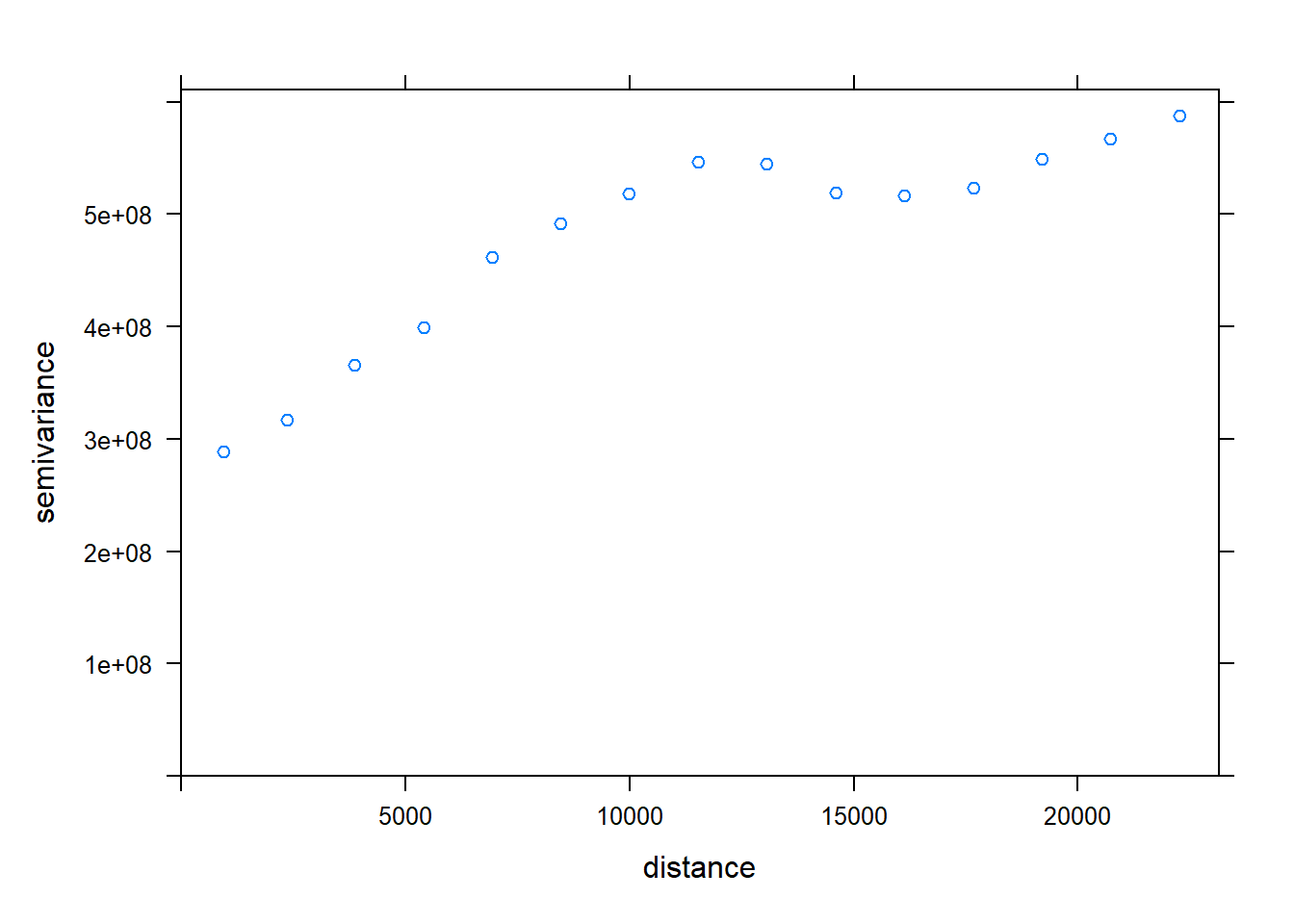
# Fit variogram
all_motor.varfit <- fit.variogram(all_motor.var,
vgm(c("Nug", "Exp")), # use vgm() to see options
fit.kappa = TRUE, fit.sills = TRUE, fit.ranges = TRUE)
plot(all_motor.var, all_motor.varfit)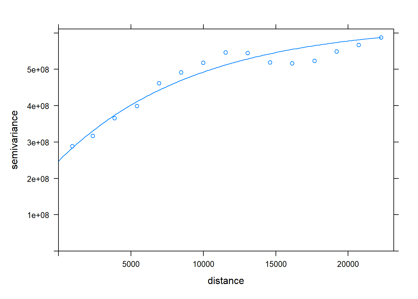
# Parameters
all_motor.varfit## model psill range
## 1 Nug 247961391 0.000
## 2 Exp 375753644 9492.608### Ordinary Kriging
#(ATTENTION: This can take some time (~3-5min with current setting))
all_motor.kg <- krige(all_motor_vehicles ~ 1,
locations = traffic.spdf,
newdata = grid,
model = all_motor.varfit)## [using ordinary kriging]# Look at results
mapview(all_motor.kg[, "var1.pred"])The example above is a little bit tricky, given that traffic does not follow a random process, but (usually) follows the street network. We would probably increase the performance by either adding the street network (e.g. using osmdata OSM Overpass API) and interpolating along this network, or by adding covariates to our prediction (Universal Kriging). With origin - destination data, we could use stplanr for routing along the street network.
Alternatively, we can use integrated nested Laplace approximation with R-INLA (Gómez-Rubio 2020).
However, lets add the predictions to our original msoa data using the st_intersection() operation as above.
# Calculate intersection
smoa_grid.int <- st_intersection(msoa.spdf, all_motor.kg)## Warning: attribute variables are assumed to be spatially constant throughout all
## geometries# average per MSOA
smoa_grid.int <- aggregate(list(traffic = smoa_grid.int$var1.pred),
by = list(MSOA11CD = smoa_grid.int$MSOA11CD),
mean)
# Merge back
msoa.spdf <- merge(msoa.spdf, smoa_grid.int, by = "MSOA11CD", all.x = TRUE)Save spatial data
# Save
save(msoa.spdf, file = "_data/msoa_spatial.RData")