3 Exercise I
\[ \newcommand{\Exp}{\mathrm{E}} \newcommand\given[1][]{\:#1\vert\:} \newcommand{\Cov}{\mathrm{Cov}} \newcommand{\Var}{\mathrm{Var}} \newcommand{\rank}{\mathrm{rank}} \newcommand{\bm}[1]{\boldsymbol{\mathbf{#1}}} \]
Required packages
Session info
R version 4.3.1 (2023-06-16 ucrt)
Platform: x86_64-w64-mingw32/x64 (64-bit)
Running under: Windows 10 x64 (build 19044)

Matrix products: default


locale:
[1] LC_COLLATE=English_United Kingdom.utf8
[2] LC_CTYPE=English_United Kingdom.utf8
[3] LC_MONETARY=English_United Kingdom.utf8
[4] LC_NUMERIC=C
[5] LC_TIME=English_United Kingdom.utf8

time zone: Europe/Berlin
tzcode source: internal

attached base packages:
[1] stats     graphics  grDevices utils     datasets  methods
[7] base

other attached packages:
[1] viridisLite_0.4.2 tmap_3.3-3        spatialreg_1.2-9
[4] Matrix_1.5-4.1    spdep_1.2-8       spData_2.3.0
[7] mapview_2.11.0    sf_1.0-13

loaded via a namespace (and not attached):
 [1] xfun_0.39          raster_3.6-23      htmlwidgets_1.6.2
 [4] lattice_0.21-8     vctrs_0.6.3        tools_4.3.1
 [7] crosstalk_1.2.0    LearnBayes_2.15.1  generics_0.1.3
[10] parallel_4.3.1     sandwich_3.0-2     stats4_4.3.1
[13] tibble_3.2.1       proxy_0.4-27       fansi_1.0.4
[16] pkgconfig_2.0.3    KernSmooth_2.23-21 satellite_1.0.4
[19] RColorBrewer_1.1-3 leaflet_2.1.2      webshot_0.5.5
[22] lifecycle_1.0.3    compiler_4.3.1     deldir_1.0-9
[25] munsell_0.5.0      terra_1.7-39       leafsync_0.1.0
[28] codetools_0.2-19   stars_0.6-1        htmltools_0.5.5
[31] class_7.3-22       pillar_1.9.0       MASS_7.3-60
[34] classInt_0.4-9     lwgeom_0.2-13      wk_0.7.3
[37] abind_1.4-5        boot_1.3-28.1      multcomp_1.4-25
[40] nlme_3.1-162       tidyselect_1.2.0   digest_0.6.32
[43] mvtnorm_1.2-2      dplyr_1.1.2        splines_4.3.1
[46] fastmap_1.1.1      grid_4.3.1         colorspace_2.1-0
[49] expm_0.999-7       cli_3.6.1          magrittr_2.0.3
[52] base64enc_0.1-3    dichromat_2.0-0.1  XML_3.99-0.14
[55] survival_3.5-5     utf8_1.2.3         TH.data_1.1-2
[58] leafem_0.2.0       e1071_1.7-13       scales_1.2.1
[61] sp_1.6-1           rmarkdown_2.23     zoo_1.8-12
[64] png_0.1-8          coda_0.19-4        evaluate_0.21
[67] knitr_1.43         tmaptools_3.1-1    s2_1.1.4
[70] rlang_1.1.1        Rcpp_1.0.10        glue_1.6.2
[73] DBI_1.1.3          rstudioapi_0.14    jsonlite_1.8.5
[76] R6_2.5.1           units_0.8-2
Reload data from pervious session
load("_data/msoa2_spatial.RData")3.1 General Exercises
- Please calculate a neighbours weights matrix of the nearest 10 neighbours (see
spdep::knearneigh()), and create a listw object using row normalization.
coords <- st_centroid(msoa.spdf)Warning: st_centroid assumes attributes are constant over
geometriesk10.nb <- knearneigh(coords, k = 10)- Can you create a map containing the City of London (MSOA11CD = “E02000001”) and its ten nearest neighbours?
i <- which(msoa.spdf$MSOA11CD == "E02000001")

# Extract neigbours
j <- k10.nb$nn[i,]

mapview(list(msoa.spdf[i,], msoa.spdf[j,]), col.regions = c("red", "blue"))- Chose another characteristics from the data (e.g. ethnic groups or house prices) and calculate global Moran’s I for it.
# Gen nb object
k10.nb <- knn2nb(k10.nb)

# Gen listw object
k10.listw <- nb2listw(k10.nb, style = "W")

# MOran test
moran.test(msoa.spdf$per_white, listw = k10.listw)
    Moran I test under randomisation

data:  msoa.spdf$per_white
weights: k10.listw

Moran I statistic standard deviate = 55.733, p-value <
2.2e-16
alternative hypothesis: greater
sample estimates:
Moran I statistic       Expectation          Variance
0.7623842505 -0.0010183299 0.0001876235 - Produce a LISA cluster map for the characteristic you have chosen.
loci2 <- localmoran(msoa.spdf$per_white, listw = k10.listw)

# Calculate clusters
msoa.spdf$lisa_cluster <- hotspot(loci2,
                                  "Pr(z != E(Ii))",
                                  cutoff = 0.05,
                                  quadrant.type = "mean",
                                  p.adjust = "BY")

# Map
mp1 <-  tm_shape(msoa.spdf) +
  tm_fill(col = c("lisa_cluster"),
          palette = viridis(n = 3, direction = -1, option = "D"),
          colorNA = "white") +
  tm_borders(col = "grey70", lwd = 0.5, alpha = 0.5) +
  tm_layout(frame = FALSE,
            legend.frame = TRUE, legend.bg.color = TRUE,
            legend.position = c("left", "bottom"),
            legend.outside = FALSE,
            main.title = "Percentage White \n LISA Clusters p(BY) < 0.05",
            main.title.position = "center",
            main.title.size = 1.6,
            legend.title.size = 0.8,
            legend.text.size = 0.8,)

mp1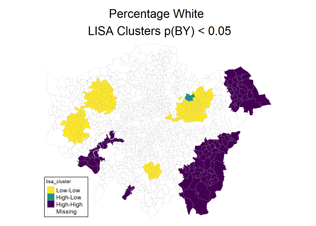
3.2 Environmental inequality
How would you investigate the following descriptive research question: Are ethnic (and immigrant) minorities in London exposed to higher levels of pollution? Also consider the spatial structure. What’s your dependent and what’s your independent variable?
1) Define a neigbours weights object of your choice
You can choose any preferred neighbours-weights definition, such as for instance contiguity neighbours or all neighbourhoods within 2.5km.
coords <- st_centroid(msoa.spdf)Warning: st_centroid assumes attributes are constant over
geometries# Neighbours within 3km distance
dist_15.nb <- dnearneigh(coords, d1 = 0, d2 = 2500)
summary(dist_15.nb)Neighbour list object:
Number of regions: 983
Number of nonzero links: 15266
Percentage nonzero weights: 1.579859
Average number of links: 15.53001
4 regions with no links:
158 463 478 505
Link number distribution:
0 1 2 3 4 5 6 7 8 9 10 11 12 13 14 15 16 17 18 19 20 21
4 5 9 23 19 26 36 31 53 39 61 63 59 48 42 35 24 31 28 30 27 26
22 23 24 25 26 27 28 29 30 31 32 33 34
25 19 38 29 32 38 26 16 20 10 8 1 2
5 least connected regions:
160 469 474 597 959 with 1 link
2 most connected regions:
565 567 with 34 links# There are some mpty one. Lets impute with the nearest neighbour
k2.nb <- knearneigh(coords, k = 1)
# Replace zero
nolink_ids <- which(card(dist_15.nb) == 0)
dist_15.nb[card(dist_15.nb) == 0] <- k2.nb$nn[nolink_ids, ]
summary(dist_15.nb)Neighbour list object:
Number of regions: 983
Number of nonzero links: 15270
Percentage nonzero weights: 1.580273
Average number of links: 15.53408
Link number distribution:
1 2 3 4 5 6 7 8 9 10 11 12 13 14 15 16 17 18 19 20 21 22
9 9 23 19 26 36 31 53 39 61 63 59 48 42 35 24 31 28 30 27 26 25
23 24 25 26 27 28 29 30 31 32 33 34
19 38 29 32 38 26 16 20 10 8 1 2
9 least connected regions:
158 160 463 469 474 478 505 597 959 with 1 link
2 most connected regions:
565 567 with 34 links# listw object with row-normalization
dist_15.lw <- nb2listw(dist_15.nb, style = "W")2) Estimate the extent of spatial auto-correlation
The most common way would be to calculate Global Moran’s I.
moran.test(msoa.spdf$no2, listw = dist_15.lw)
    Moran I test under randomisation

data:  msoa.spdf$no2
weights: dist_15.lw

Moran I statistic standard deviate = 65.197, p-value <
2.2e-16
alternative hypothesis: greater
sample estimates:
Moran I statistic       Expectation          Variance
      0.891520698      -0.001018330       0.000187411