1  Refresher

Required packages

pkgs <- c("sf", "gstat", "mapview", "nngeo", "rnaturalearth", "dplyr",
          "nomisr", "osmdata", "tidyr", "texreg") 
lapply(pkgs, require, character.only = TRUE)

Session info

sessionInfo()

R version 4.3.1 (2023-06-16 ucrt)
Platform: x86_64-w64-mingw32/x64 (64-bit)
Running under: Windows 10 x64 (build 19044)

Matrix products: default


locale:
[1] LC_COLLATE=English_United Kingdom.utf8 
[2] LC_CTYPE=English_United Kingdom.utf8   
[3] LC_MONETARY=English_United Kingdom.utf8
[4] LC_NUMERIC=C                           
[5] LC_TIME=English_United Kingdom.utf8    

time zone: Europe/Berlin
tzcode source: internal

attached base packages:
[1] stats     graphics  grDevices utils     datasets  methods  
[7] base     

other attached packages:
 [1] texreg_1.38.6       tidyr_1.3.0         osmdata_0.2.3      
 [4] nomisr_0.4.7        dplyr_1.1.2         rnaturalearth_0.3.3
 [7] nngeo_0.4.7         mapview_2.11.0      gstat_2.1-1        
[10] sf_1.0-13          

loaded via a namespace (and not attached):
 [1] xfun_0.39          raster_3.6-23      htmlwidgets_1.6.2 
 [4] lattice_0.21-8     vctrs_0.6.3        tools_4.3.1       
 [7] crosstalk_1.2.0    generics_0.1.3     stats4_4.3.1      
[10] tibble_3.2.1       proxy_0.4-27       spacetime_1.3-0   
[13] fansi_1.0.4        xts_0.13.1         pkgconfig_2.0.3   
[16] KernSmooth_2.23-21 satellite_1.0.4    data.table_1.14.8 
[19] leaflet_2.1.2      webshot_0.5.5      lifecycle_1.0.3   
[22] compiler_4.3.1     FNN_1.1.3.2        rsdmx_0.6-2       
[25] munsell_0.5.0      terra_1.7-39       codetools_0.2-19  
[28] snakecase_0.11.0   htmltools_0.5.5    class_7.3-22      
[31] pillar_1.9.0       classInt_0.4-9     tidyselect_1.2.0  
[34] digest_0.6.32      purrr_1.0.1        fastmap_1.1.1     
[37] grid_4.3.1         colorspace_2.1-0   cli_3.6.1         
[40] magrittr_2.0.3     base64enc_0.1-3    XML_3.99-0.14     
[43] utf8_1.2.3         leafem_0.2.0       e1071_1.7-13      
[46] scales_1.2.1       sp_1.6-1           rmarkdown_2.23    
[49] httr_1.4.6         zoo_1.8-12         png_0.1-8         
[52] evaluate_0.21      knitr_1.43         rlang_1.1.1       
[55] Rcpp_1.0.10        glue_1.6.2         DBI_1.1.3         
[58] rstudioapi_0.14    jsonlite_1.8.5     R6_2.5.1          
[61] plyr_1.8.8         intervals_0.15.4   units_0.8-2       

1.1 Packages

Please make sure that you have installed the following packages:

pks <- c("dplyr",
"gstat",
"mapview",
"nngeo",
"nomisr",
"osmdata",
"rnaturalearth",
"sf",
"spatialreg",
"spdep",
"texreg",
"tidyr",
"tmap",
"viridisLite")

The most important package is sf: Simple Features for R. users are strongly encouraged to install the sf binary packages from CRAN. If that does not work, please have a look at the installation instructions. It requires software packages GEOS, GDAL and PROJ.

1.2 Coordinates

In general, spatial data is structured like conventional/tidy data (e.g. data.frames, matrices), but has one additional dimension: every observation is linked to some sort of geo-spatial information. Most common types of spatial information are:

• Points (one coordinate pair)

• Lines (two coordinate pairs)

• Polygons (at least three coordinate pairs)

• Regular grids (one coordinate pair for centroid + raster / grid size)

1.2.1 Coordinate reference system (CRS)

In its raw form, a pair of coordinates consists of two numerical values. For instance, the pair c(51.752595, -1.262801) describes the location of Nuffield College in Oxford (one point). The fist number represents the latitude (north-south direction), the second number is the longitude (west-east direction), both are in decimal degrees.

Figure: Latitude and longitude, Source: Wikipedia

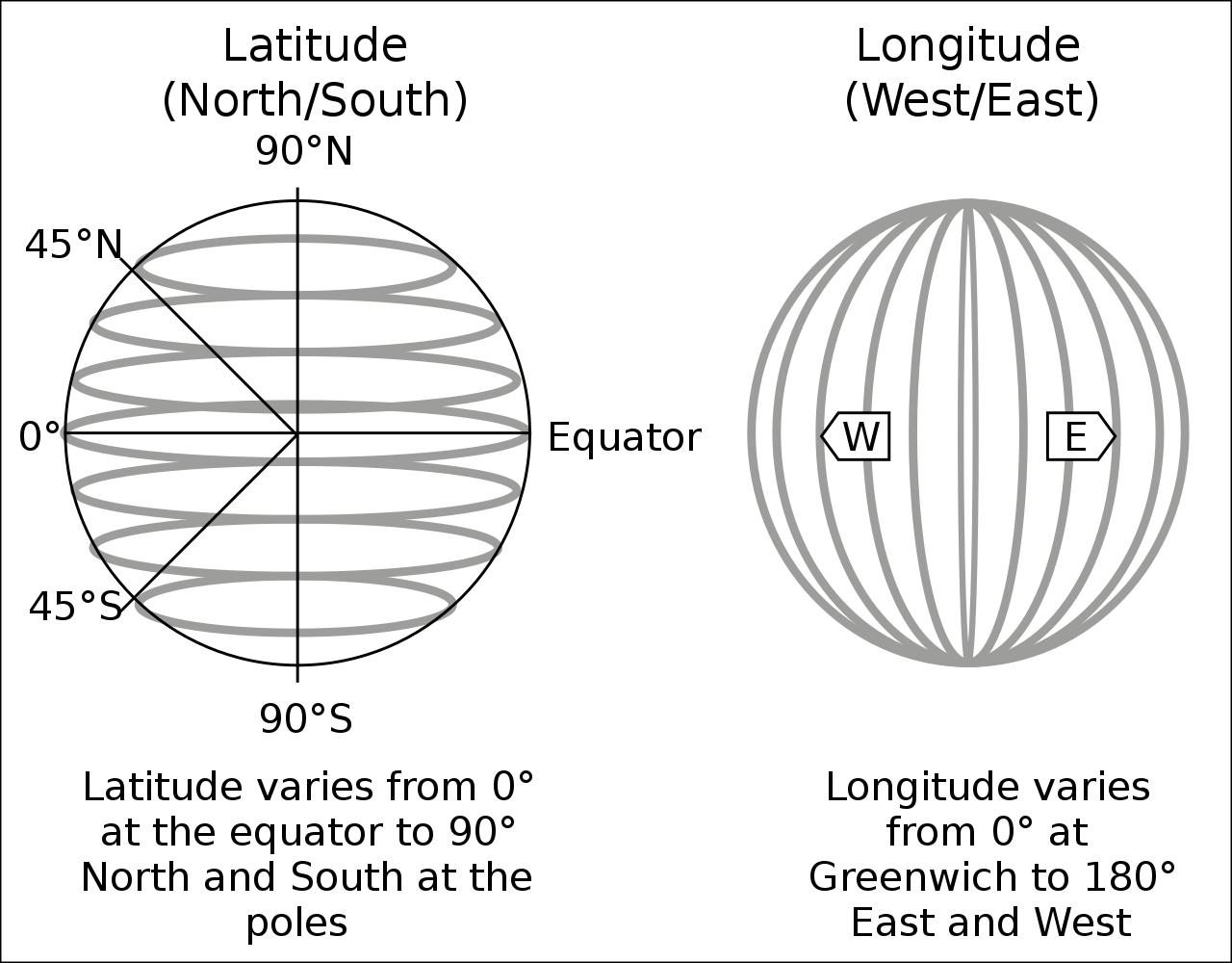
However, we need to specify a reference point for latitudes and longitudes (in the Figure above: equator and Greenwich). For instance, the pair of coordinates above comes from Google Maps which returns GPS coordinates in ‘WGS 84’ (EPSG:4326).

# Coordinate pairs of two locations
coords1 <- c(51.752595, -1.262801)
coords2 <- c(51.753237, -1.253904)
coords <- rbind(coords1, coords2)

# Conventional data frame
nuffield.df <- data.frame(name = c("Nuffield College", "Radcliffe Camera"),
                          address = c("New Road", "Radcliffe Sq"),
                          lat = coords[,1], lon = coords[,2])

head(nuffield.df)

                    name      address      lat       lon
coords1 Nuffield College     New Road 51.75259 -1.262801
coords2 Radcliffe Camera Radcliffe Sq 51.75324 -1.253904

# Combine to spatial data frame
nuffield.spdf <- st_as_sf(nuffield.df, 
                          coords = c("lon", "lat"), # Order is important
                          crs = 4326) # EPSG number of CRS

# Map
mapview(nuffield.spdf, zcol = "name")

1.2.2 Projected CRS

However, different data providers use different CRS. For instance, spatial data in the UK usually uses ‘OSGB 1936 / British National Grid’ (EPSG:27700). Here, coordinates are in meters, and projected onto a planar 2D space.

There are a lot of different CRS projections, and different national statistics offices provide data in different projections. Data providers usually specify which reference system they use. This is important as using the correct reference system and projection is crucial for plotting and manipulating spatial data.

If you do not know the correct CRS, try starting with a standards CRS like EPSG:4326 if you have decimal degree like coordinates. If it looks like projected coordinates, try searching for the country or region in CRS libraries like https://epsg.io/. However, you must check if the projected coordinates match their real location, e.g. using mapview().

1.2.3 Why different projections?

By now, (most) people agree that the earth is not flat. So, to plot data on a 2D planar surface and to perform certain operations on a planar world, we need to make some re-projections. Depending on where we are, different re-projections of our data (globe in this case) might work better than others.

world <- ne_countries(scale = "medium", returnclass = "sf")
class(world)

[1] "sf"         "data.frame"

st_crs(world)

Coordinate Reference System:
  User input: +proj=longlat +datum=WGS84 +no_defs +ellps=WGS84 +towgs84=0,0,0 
  wkt:
BOUNDCRS[
    SOURCECRS[
        GEOGCRS["unknown",
            DATUM["World Geodetic System 1984",
                ELLIPSOID["WGS 84",6378137,298.257223563,
                    LENGTHUNIT["metre",1]],
                ID["EPSG",6326]],
            PRIMEM["Greenwich",0,
                ANGLEUNIT["degree",0.0174532925199433],
                ID["EPSG",8901]],
            CS[ellipsoidal,2],
                AXIS["longitude",east,
                    ORDER[1],
                    ANGLEUNIT["degree",0.0174532925199433,
                        ID["EPSG",9122]]],
                AXIS["latitude",north,
                    ORDER[2],
                    ANGLEUNIT["degree",0.0174532925199433,
                        ID["EPSG",9122]]]]],
    TARGETCRS[
        GEOGCRS["WGS 84",
            DATUM["World Geodetic System 1984",
                ELLIPSOID["WGS 84",6378137,298.257223563,
                    LENGTHUNIT["metre",1]]],
            PRIMEM["Greenwich",0,
                ANGLEUNIT["degree",0.0174532925199433]],
            CS[ellipsoidal,2],
                AXIS["latitude",north,
                    ORDER[1],
                    ANGLEUNIT["degree",0.0174532925199433]],
                AXIS["longitude",east,
                    ORDER[2],
                    ANGLEUNIT["degree",0.0174532925199433]],
            ID["EPSG",4326]]],
    ABRIDGEDTRANSFORMATION["Transformation from unknown to WGS84",
        METHOD["Geocentric translations (geog2D domain)",
            ID["EPSG",9603]],
        PARAMETER["X-axis translation",0,
            ID["EPSG",8605]],
        PARAMETER["Y-axis translation",0,
            ID["EPSG",8606]],
        PARAMETER["Z-axis translation",0,
            ID["EPSG",8607]]]]

# Extract a country and plot in current CRS (WGS84)
ger.spdf <- world[world$name == "Germany", ]
plot(st_geometry(ger.spdf))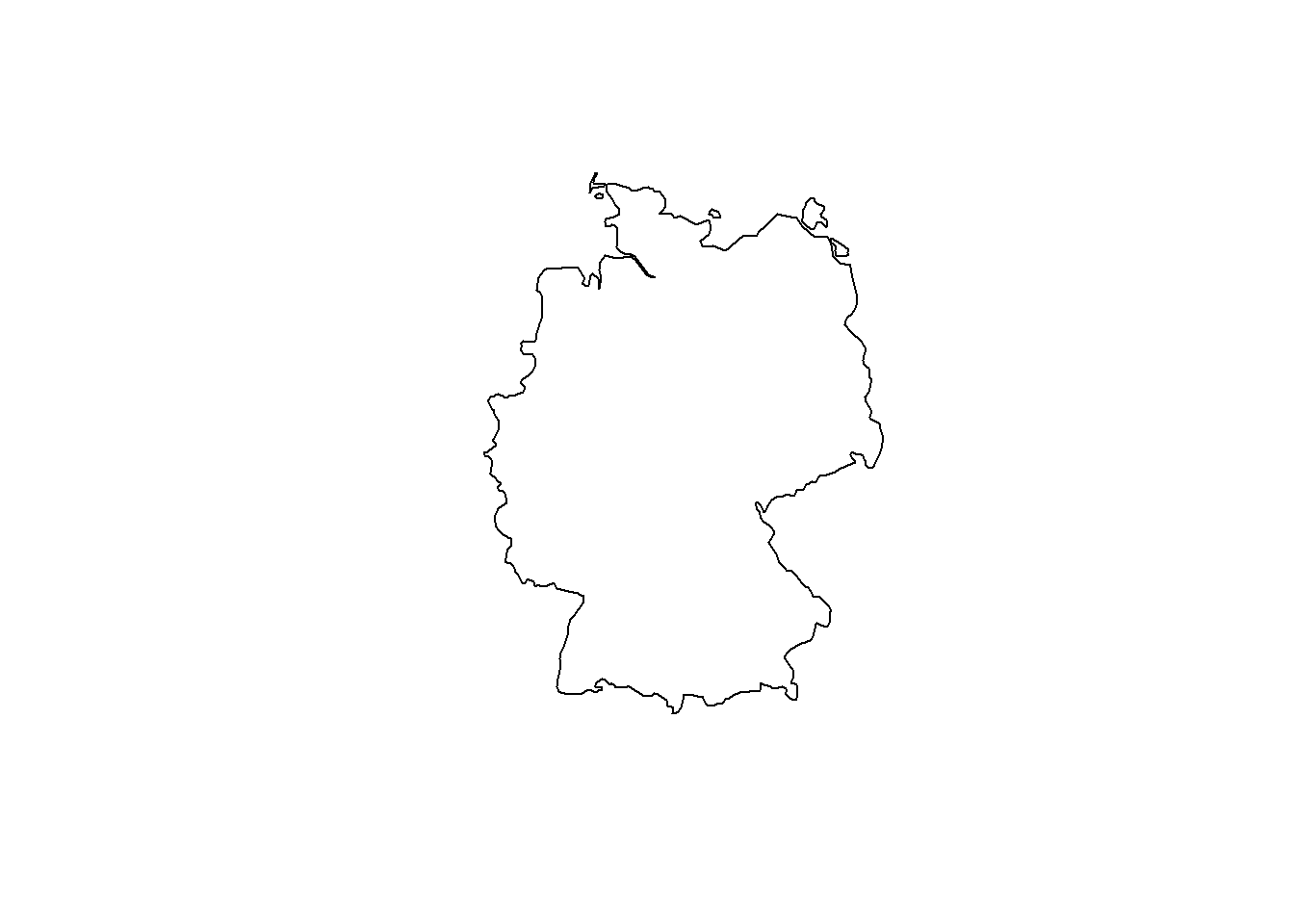

# Now, let's transform Germany into a CRS optimized for Iceland
ger_rep.spdf <- st_transform(ger.spdf, crs = 5325)
plot(st_geometry(ger_rep.spdf))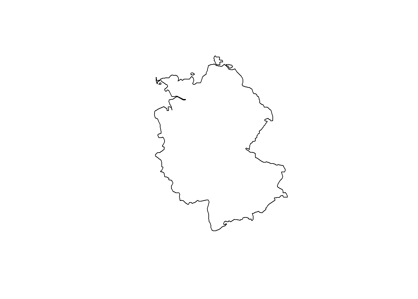

Depending on the angle, a 2D projection of the earth looks different. It is important to choose a suitable projection for the available spatial data. For more information on CRS and re-projection, see e.g. Lovelace, Nowosad, and Muenchow (2019) or Stefan Jünger & Anne-Kathrin Stroppe’s GESIS workshop materials.

1.3 Importing some real world data

sf imports many of the most common spatial data files, like geojson, gpkg, or shp.

1.3.1 London shapefile (polygon)

Let’s get some administrative boundaries for London from the London Datastore. We use the sf package and its funtion st_read() to import the data.

# Create subdir (all data withh be stored in "_data")
dn <- "_data"
ifelse(dir.exists(dn), "Exists", dir.create(dn))

[1] "Exists"

# Download zip file and unzip
tmpf <- tempfile()
boundary.link <- "https://data.london.gov.uk/download/statistical-gis-boundary-files-london/9ba8c833-6370-4b11-abdc-314aa020d5e0/statistical-gis-boundaries-london.zip"
download.file(boundary.link, tmpf)
unzip(zipfile = tmpf, exdir = paste0(dn))
unlink(tmpf)

# This is a shapefile
# We only need the MSOA layer for now
msoa.spdf <- st_read(dsn = paste0(dn, "/statistical-gis-boundaries-london/ESRI"),
                     layer = "MSOA_2011_London_gen_MHW" # Note: no file ending
                     )

Reading layer `MSOA_2011_London_gen_MHW' from data source 
  `C:\work\Lehre\Geodata_Spatial_Regression_short\_data\statistical-gis-boundaries-london\ESRI' 
  using driver `ESRI Shapefile'
Simple feature collection with 983 features and 12 fields
Geometry type: MULTIPOLYGON
Dimension:     XY
Bounding box:  xmin: 503574.2 ymin: 155850.8 xmax: 561956.7 ymax: 200933.6
Projected CRS: OSGB36 / British National Grid

The object msoa.spdf is our spatial data.frame. It looks essentially like a conventional data.frame, but has some additional attributes and geo-graphical information stored with it. Most importantly, notice the column geometry, which contains a list of polygons. In most cases, we have one polygon for each line / observation.

head(msoa.spdf)

Simple feature collection with 6 features and 12 fields
Geometry type: MULTIPOLYGON
Dimension:     XY
Bounding box:  xmin: 530966.7 ymin: 180510.7 xmax: 551943.8 ymax: 191139
Projected CRS: OSGB36 / British National Grid
   MSOA11CD                 MSOA11NM   LAD11CD              LAD11NM
1 E02000001       City of London 001 E09000001       City of London
2 E02000002 Barking and Dagenham 001 E09000002 Barking and Dagenham
3 E02000003 Barking and Dagenham 002 E09000002 Barking and Dagenham
4 E02000004 Barking and Dagenham 003 E09000002 Barking and Dagenham
5 E02000005 Barking and Dagenham 004 E09000002 Barking and Dagenham
6 E02000007 Barking and Dagenham 006 E09000002 Barking and Dagenham
    RGN11CD RGN11NM USUALRES HHOLDRES COMESTRES POPDEN HHOLDS
1 E12000007  London     7375     7187       188   25.5   4385
2 E12000007  London     6775     6724        51   31.3   2713
3 E12000007  London    10045    10033        12   46.9   3834
4 E12000007  London     6182     5937       245   24.8   2318
5 E12000007  London     8562     8562         0   72.1   3183
6 E12000007  London     8791     8672       119   50.6   3441
  AVHHOLDSZ                       geometry
1       1.6 MULTIPOLYGON (((531667.6 18...
2       2.5 MULTIPOLYGON (((548881.6 19...
3       2.6 MULTIPOLYGON (((549102.4 18...
4       2.6 MULTIPOLYGON (((551550 1873...
5       2.7 MULTIPOLYGON (((549099.6 18...
6       2.5 MULTIPOLYGON (((549819.9 18...

Shapefiles are still among the most common formats to store and transmit spatial data, despite them being inefficient (file size and file number).

However, sf reads everything spatial, such as geo.json, which usually is more efficient, but less common (but we’re getting there).

# Download file
ulez.link <- "https://data.london.gov.uk/download/ultra_low_emissions_zone/936d71d8-c5fc-40ad-a392-6bec86413b48/CentralUltraLowEmissionZone.geojson"
download.file(ulez.link, paste0(dn, "/ulez.json"))

# Read geo.json
st_layers(paste0(dn, "/ulez.json"))

Driver: GeoJSON 
Available layers:
                   layer_name geometry_type features fields
1 CentralUltraLowEmissionZone Multi Polygon        1      4
                        crs_name
1 OSGB36 / British National Grid

ulez.spdf <- st_read(dsn = paste0(dn, "/ulez.json")) # here dsn is simply the file

Reading layer `CentralUltraLowEmissionZone' from data source 
  `C:\work\Lehre\Geodata_Spatial_Regression_short\_data\ulez.json' 
  using driver `GeoJSON'
Simple feature collection with 1 feature and 4 fields
Geometry type: MULTIPOLYGON
Dimension:     XY
Bounding box:  xmin: 527271.5 ymin: 178041.5 xmax: 533866.3 ymax: 183133.4
Projected CRS: OSGB36 / British National Grid

head(ulez.spdf)

Simple feature collection with 1 feature and 4 fields
Geometry type: MULTIPOLYGON
Dimension:     XY
Bounding box:  xmin: 527271.5 ymin: 178041.5 xmax: 533866.3 ymax: 183133.4
Projected CRS: OSGB36 / British National Grid
  fid OBJECTID BOUNDARY Shape_Area                       geometry
1   1        1 CSS Area   21.37557 MULTIPOLYGON (((531562.7 18...

Again, this looks like a conventional data.frame but has the additional column geometry containing the coordinates of each observation. st_geometry() returns only the geographic object and st_drop_geometry() only the data.frame without the coordinates. We can plot the object using mapview().

mapview(msoa.spdf[, "POPDEN"])

1.3.2 Census API (admin units)

Now that we have some boundaries and shapes of spatial units in London, we can start looking for different data sources to populate the geometries.

A good source for demographic data is for instance the 2011 census. Below we use the nomis API to retrieve population data for London, See the Vignette for more information (Guest users are limited to 25,000 rows per query). Below is a wrapper to avoid some errors with sex and urban-rural cross-tabulation in some of the data.

### For larger request, register and set key
# Sys.setenv(NOMIS_API_KEY = "XXX")
# nomis_api_key(check_env = TRUE)

x <- nomis_data_info()

# Get London ids
london_ids <- msoa.spdf$MSOA11CD

### Get key statistics ids
# select requires tables (https://www.nomisweb.co.uk/sources/census_2011_ks)
# Let's get KS201EW (ethnic group), KS205EW (passport held), and KS402EW (housing tenure)

# Get internal ids
stats <- c("KS201EW", "KS402EW", "KS205EW")
oo <- which(grepl(paste(stats, collapse = "|"), x$name.value))
ksids <- x$id[oo]
ksids # This are the internal ids

[1] "NM_608_1" "NM_612_1" "NM_619_1"

### look at meta information
q <- nomis_overview(ksids[1])
head(q)

# A tibble: 6 × 2
  name           value           
  <chr>          <list>          
1 analyses       <named list [1]>
2 analysisname   <chr [1]>       
3 analysisnumber <int [1]>       
4 contact        <named list [4]>
5 contenttypes   <named list [1]>
6 coverage       <chr [1]>       

a <- nomis_get_metadata(id = ksids[1], concept = "GEOGRAPHY", type = "type")
a # TYPE297 is MSOA level

# A tibble: 24 × 3
   id      label.en                                   description.en
   <chr>   <chr>                                      <chr>         
 1 TYPE265 NHS area teams                             NHS area teams
 2 TYPE266 clinical commissioning groups              clinical comm…
 3 TYPE267 built-up areas including subdivisions      built-up area…
 4 TYPE269 built-up areas                             built-up areas
 5 TYPE273 national assembly for wales electoral reg… national asse…
 6 TYPE274 postcode areas                             postcode areas
 7 TYPE275 postcode districts                         postcode dist…
 8 TYPE276 postcode sectors                           postcode sect…
 9 TYPE277 national assembly for wales constituencie… national asse…
10 TYPE279 parishes 2011                              parishes 2011 
# ℹ 14 more rows

b <- nomis_get_metadata(id = ksids[1], concept = "MEASURES", type = "TYPE297")
b # 20100 is the measure of absolute numbers

# A tibble: 2 × 3
  id    label.en description.en
  <chr> <chr>    <chr>         
1 20100 value    value         
2 20301 percent  percent       

### Query data in loop over the required statistics
for(i in ksids){

  # Determin if data is divided by sex or urban-rural
  nd <- nomis_get_metadata(id = i)
  if("RURAL_URBAN" %in% nd$conceptref){
    UR <- TRUE
  }else{
    UR <- FALSE
  }
  if("C_SEX" %in% nd$conceptref){
    SEX <- TRUE
  }else{
    SEX <- FALSE
  }

  # make data request
  if(UR == TRUE){
    if(SEX == TRUE){
      tmp_en <- nomis_get_data(id = i, time = "2011",
                               geography = london_ids, # replace with "TYPE297" for all MSOAs
                               measures = 20100, RURAL_URBAN = 0, C_SEX = 0)
    }else{
      tmp_en <- nomis_get_data(id = i, time = "2011",
                               geography = london_ids, # replace with "TYPE297" for all MSOAs
                               measures = 20100, RURAL_URBAN = 0)
    }
  }else{
    if(SEX == TRUE){
      tmp_en <- nomis_get_data(id = i, time = "2011",
                               geography = london_ids, # replace with "TYPE297" for all MSOAs
                               measures = 20100, C_SEX = 0)
    }else{
      tmp_en <- nomis_get_data(id = i, time = "2011",
                               geography = london_ids, # replace with "TYPE297" for all MSOAs
                               measures = 20100)
    }

  }

  # Append (in case of different regions)
  ks_tmp <- tmp_en

  # Make lower case names
  names(ks_tmp) <- tolower(names(ks_tmp))
  names(ks_tmp)[names(ks_tmp) == "geography_code"] <- "msoa11"
  names(ks_tmp)[names(ks_tmp) == "geography_name"] <- "name"

  # replace weird cell codes
  onlynum <- which(grepl("^[[:digit:]]+$", ks_tmp$cell_code))
  if(length(onlynum) != 0){
    code <- substr(ks_tmp$cell_code[-onlynum][1], 1, 7)
    if(is.na(code)){
      code <- i
    }
    ks_tmp$cell_code[onlynum] <- paste0(code, "_", ks_tmp$cell_code[onlynum])
  }

  # save codebook
  ks_cb <- unique(ks_tmp[, c("date", "cell_type", "cell", "cell_code", "cell_name")])

  ### Reshape
  ks_res <- tidyr::pivot_wider(ks_tmp, id_cols = c("msoa11", "name"),
                               names_from = "cell_code",
                               values_from = "obs_value")

  ### Merge
  if(i == ksids[1]){
    census_keystat.df <- ks_res
    census_keystat_cb.df <- ks_cb
  }else{
    census_keystat.df <- merge(census_keystat.df, ks_res, by = c("msoa11", "name"), all = TRUE)
    census_keystat_cb.df <- rbind(census_keystat_cb.df, ks_cb)
  }

}


# Descriptions are saved in the codebook
head(census_keystat_cb.df)

# A tibble: 6 × 5
   date cell_type     cell cell_code   cell_name                    
  <dbl> <chr>        <dbl> <chr>       <chr>                        
1  2011 Ethnic Group     0 KS201EW0001 All usual residents          
2  2011 Ethnic Group   100 KS201EW_100 White                        
3  2011 Ethnic Group     1 KS201EW0002 White: English/Welsh/Scottis…
4  2011 Ethnic Group     2 KS201EW0003 White: Irish                 
5  2011 Ethnic Group     3 KS201EW0004 White: Gypsy or Irish Travel…
6  2011 Ethnic Group     4 KS201EW0005 White: Other White           

save(census_keystat_cb.df, file = "_data/Census_codebook.RData")

Now, we have one file containing the geometries of MSOAs and one file with the census information on ethnic groups. Obviously, we can easily merge them together using the MSOA identifiers.

msoa.spdf <- merge(msoa.spdf, census_keystat.df,
                   by.x = "MSOA11CD", by.y = "msoa11", all.x = TRUE)

And we can, for instance, plot the spatial distribution of ethnic groups.

msoa.spdf$per_white <- msoa.spdf$KS201EW_100 / msoa.spdf$KS201EW0001 * 100
msoa.spdf$per_mixed <- msoa.spdf$KS201EW_200 / msoa.spdf$KS201EW0001 * 100
msoa.spdf$per_asian <- msoa.spdf$KS201EW_300 / msoa.spdf$KS201EW0001 * 100
msoa.spdf$per_black <- msoa.spdf$KS201EW_400 / msoa.spdf$KS201EW0001 * 100
msoa.spdf$per_other <- msoa.spdf$KS201EW_500 / msoa.spdf$KS201EW0001 * 100

mapview(msoa.spdf[, "per_white"])

If you’re interested in more data sources, see for instance APIs for social scientists: A collaborative review by Paul C. Bauer, Camille Landesvatter, Lion Behrens. It’s a collection of several APIs for social sciences.

1.3.3 Gridded data

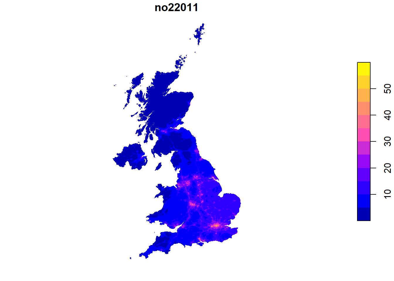
So far, we have queried data on administrative units. However, often data comes on other spatial scales. For instance, we might be interested in the amount of air pollution, which is provided on a regular grid across the UK from Defra.

# Download
pol.link <- "https://uk-air.defra.gov.uk/datastore/pcm/mapno22011.csv"
download.file(pol.link, paste0(dn, "/mapno22011.csv"))
pol.df <- read.csv(paste0(dn, "/mapno22011.csv"), skip = 5, header = T, sep = ",",
                      stringsAsFactors = F, na.strings = "MISSING")

head(pol.df)

  ukgridcode      x       y no22011
1      54291 460500 1221500      NA
2      54292 461500 1221500      NA
3      54294 463500 1221500      NA
4      54979 458500 1220500      NA
5      54980 459500 1220500      NA
6      54981 460500 1220500      NA

The data comes as point data with x and y as coordinates. We have to transform this into spatial data first. We first setup a spatial points object with st_as_sf. Subsequently, we transform the point coordinates into a regular grid. We use a buffer method st_buffer with “diameter”, and only one segment per quadrant (nQuadSegs). This gives us a 1x1km regular grid.

# Build spatial object
pol.spdf <- st_as_sf(pol.df, coords = c("x", "y"),
                    crs = 27700)

# we transform the point coordinates into a regular grid with "diameter" 500m
pol.spdf <- st_buffer(pol.spdf, dist = 500, nQuadSegs  = 1,
                      endCapStyle = 'SQUARE')

# Plot NO2
plot(pol.spdf[, "no22011"], border = NA)

1.3.4 OpenStreetMap (points)

Another interesting data source is the OpenStreetMap API, which provides information about the geographical location of a serious of different indicators. Robin Lovelace provides a nice introduction to the osmdata API. Available features can be found on OSM wiki.

First we create a bounding box of where we want to query data. st_bbox() can be used to get bounding boxes of an existing spatial object (needs CRS = 4326). An alternative would be to use opq(bbox = 'greater london uk').

# bounding box of where we want to query data
q <- opq(bbox = st_bbox(st_transform(msoa.spdf, 4326)))

And we want to get data for all pubs and bars which are within this bounding box.

# First build the query of location of pubs in London
osmq <- add_osm_feature(q, key = "amenity", value = "pub")

# And then query the data
pubs.osm <- osmdata_sf(osmq)

Right now there are some results in polygons, some in points, and they overlap. Often, data from OSM needs some manual cleaning. Sometimes the same features are represented by different spatial objects (e.g. points + polygons).

# Make unique points / polygons
pubs.osm <- unique_osmdata(pubs.osm)

# Get points and polygons (there are barley any pubs as polygons, so we ignore them)
pubs.points <- pubs.osm$osm_points
pubs.polys <- pubs.osm$osm_multipolygons

# # Drop OSM file
# rm(pubs.osm); gc()

# Reduce to point object only
pubs.spdf <- pubs.points

# Reduce to a few variables
pubs.spdf <- pubs.spdf[, c("osm_id", "name", "addr:postcode", "diet:vegan")]

Again, we can inspect the results with mapview.

mapview(st_geometry(pubs.spdf))

Note that OSM is solely based on contribution by users, and the quality of OSM data varies. Usually data quality is better in larger cities, and better for more stable features (such as hospitals, train stations, highways) rahter than pubs or restaurants which regularly appear and disappear. However, data from London Datastore would indicate more pubs than what we find with OSM.

1.3.5 Save

We will store the created data to use them again in the next session.

save(msoa.spdf, file = "_data/msoa_spatial.RData")
save(ulez.spdf, file = "_data/ulez_spatial.RData")
save(pol.spdf, file = "_data/pollution_spatial.RData")
save(pubs.spdf, file = "_data/pubs_spatial.RData")

1.4 Data Manipulation

Required packages

pkgs <- c("sf", "gstat", "mapview", "nngeo", "rnaturalearth", "dplyr",
          "nomisr", "osmdata", "tidyr", "texreg", "downlit", "xml2") 
lapply(pkgs, require, character.only = TRUE)

Having data with geo-spatial information allows to perform a variety of methods to manipulate and link different data sources. Commonly used methods include 1) subsetting, 2) point-in-polygon operations, 3) distance measures, 4) intersections or buffer methods.

The online Vignettes of the sf package provide a comprehensive overview of the multiple ways of spatial manipulations.

Check if data is on common projection

st_crs(msoa.spdf) == st_crs(pol.spdf)

[1] FALSE

st_crs(msoa.spdf) == st_crs(pubs.spdf)

[1] FALSE

st_crs(msoa.spdf) == st_crs(ulez.spdf)

[1] FALSE

The spatial data files are on different projections. Before we can do any spatial operations with them, we have to transform them into a common projection.

# MSOA in different crs --> transform
pol.spdf <- st_transform(pol.spdf, crs = st_crs(msoa.spdf))
pubs.spdf <- st_transform(pubs.spdf, crs = st_crs(msoa.spdf))
ulez.spdf <- st_transform(ulez.spdf, crs = st_crs(msoa.spdf))


# Check if all geometries are valid, and make valid if needed
msoa.spdf <- st_make_valid(msoa.spdf)

The st_make_valid() can help if the spatial geometries have some problems such as holes or points that don’t match exactly.

1.4.1 Subsetting

We can subset spatial data in a similar way as we subset conventional data.frames or matrices. For instance, below we simply reduce the pollution grid across the UK to observations in London only.

# Subset to pollution estimates in London
pol_sub.spdf <- pol.spdf[msoa.spdf, ] # or:
pol_sub.spdf <- st_filter(pol.spdf, msoa.spdf)
mapview(pol_sub.spdf)

Or we can reverse the above and exclude all intersecting units by specifying st_disjoint as alternative spatial operation using the op = option (note the empty space for column selection). st_filter() with the .predicate option does the same job. See the sf Vignette for more operations.

# Subset pubs to pubs not in the ulez area
sub2.spdf <- pubs.spdf[ulez.spdf, , op = st_disjoint] # or:
sub2.spdf <- st_filter(pubs.spdf, ulez.spdf, .predicate = st_disjoint)
mapview(sub2.spdf)

We can easily create indicators of whether an MSOA is within ulez or not.

msoa.spdf$ulez <- 0

# intersecting lsoas
within <- msoa.spdf[ulez.spdf,]

# use their ids to create binary indicator 
msoa.spdf$ulez[which(msoa.spdf$MSOA11CD %in% within$MSOA11CD)] <- 1
table(msoa.spdf$ulez)

  0   1 
955  28 

1.4.2 Point in polygon

We are interested in the number of pubs in each MSOA. So, we count the number of points in each polygon.

# Assign MSOA to each point
pubs_msoa.join <- st_join(pubs.spdf, msoa.spdf, join = st_within)

# Count N by MSOA code (drop geometry to speed up)
pubs_msoa.join <- dplyr::count(st_drop_geometry(pubs_msoa.join),
                               MSOA11CD = pubs_msoa.join$MSOA11CD,
                               name = "pubs_count")
sum(pubs_msoa.join$pubs_count)

[1] 1601

# Merge and replace NAs with zero (no matches, no pubs)
msoa.spdf <- merge(msoa.spdf, pubs_msoa.join,
                   by = "MSOA11CD", all.x = TRUE)
msoa.spdf$pubs_count[is.na(msoa.spdf$pubs_count)] <- 0

1.4.3 Distance measures

We might be interested in the distance to the nearest pub. Here, we use the package nngeo to find k nearest neighbours with the respective distance.

# Use geometric centroid of each MSOA
cent.sp <- st_centroid(msoa.spdf[, "MSOA11CD"])

Warning: st_centroid assumes attributes are constant over
geometries

# Get K nearest neighbour with distance
knb.dist <- st_nn(cent.sp, 
                  pubs.spdf,
                  k = 1,             # number of nearest neighbours
                  returnDist = TRUE, # we also want the distance
                  progress = FALSE)

projected points

msoa.spdf$dist_pubs <- unlist(knb.dist$dist)
summary(msoa.spdf$dist_pubs)

    Min.  1st Qu.   Median     Mean  3rd Qu.     Max. 
   9.079  305.149  565.018  701.961  948.047 3735.478 

1.4.4 Intersections + Buffers

We may also want the average pollution within 1 km radius around each MSOA centroid. Note that it is usually better to use a ego-centric method where you calculate the average within a distance rather than using the characteristic of the intersecting cells only (Lee et al. 2008; Mohai and Saha 2007).

Therefore, we first create a buffer with st_buffer() around each midpoint and subsequently use st_intersetion() to calculate the overlap.

# Create buffer (1km radius)
cent.buf <- st_buffer(cent.sp, 
                      dist = 1000) # dist in meters
mapview(cent.buf)

# Add area of each buffer (in this constant) 
cent.buf$area <- as.numeric(st_area(cent.buf))

# Calculate intersection of pollution grid and buffer
int.df <- st_intersection(cent.buf, pol.spdf)

Warning: attribute variables are assumed to be spatially constant
throughout all geometries

int.df$int_area <- as.numeric(st_area(int.df)) # area of intersection

# Area of intersection as share of buffer
int.df$area_per <- int.df$int_area / int.df$area

And we use the percent overalp areas as the weights to calculate a weighted mean.

# Aggregate as weighted mean
int.df <- st_drop_geometry(int.df)
int.df$no2_weighted <- int.df$no22011 * int.df$area_per
int.df <- aggregate(list(no2 = int.df[, "no2_weighted"]), 
                    by = list(MSOA11CD = int.df$MSOA11CD),
                    sum)

# Merge back to spatial data.frame
msoa.spdf <- merge(msoa.spdf, int.df, by = "MSOA11CD", all.x = TRUE)

mapview(msoa.spdf[, "no2"])

Note: for buffer related methods, it often makes sense to use population weighted centroids instead of geographic centroids (see here for MSOA population weighted centroids). However, often this information is not available.

1.4.5 and more

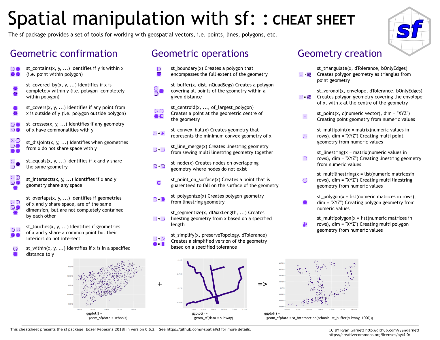
There are more spatial operation possible using sf. Have a look at the sf Cheatsheet.

1.5 Data visualisation

For mapping

pkgs <- c("tmap", "tmaptools", "viridisLite", 
          "ggplot2", "ggthemes", "rmapshaper") 
lapply(pkgs, require, character.only = TRUE)

A large advantage of spatial data is that different data sources can be connected and combined. Another nice advantage is: you can create very nice maps. And it’s quite easy to do! Stefan Jünger & Anne-Kathrin Stroppe provide more comprehensive materials on mapping in their GESIS workshop on geospatial techniques in R.

Many packages and functions can be used to plot maps of spatial data. For instance, ggplot as a function to plot spatial data using geom_sf(). I am personally a fan of tmap, which makes many steps easier (but sometimes is less flexible).

A great tool for choosing coulour is for instance Colorbrewer. viridisLite provides another great resource to chose colours.

1.5.1 Tmaps

For instance, lets plot the NO2 estimates using tmap + tm_fill() (there are lots of alternatives like tm_shape, tm_points(), tm_dots()).

# Define colours
cols <- viridis(n = 7, direction = 1, option = "C")

mp1 <-  tm_shape(msoa.spdf) + 
  tm_fill(col = "no2", 
          style = "fisher", # algorithm to def cut points
          n = 7, # Number of requested cut points
          palette = cols, # colours
          alpha = 1, # transparency 
          title = "NO2", 
          legend.hist = FALSE # histogram next to map?
          ) +
  tm_borders(col = "white", lwd = 0.5, alpha = 0.5) 

mp1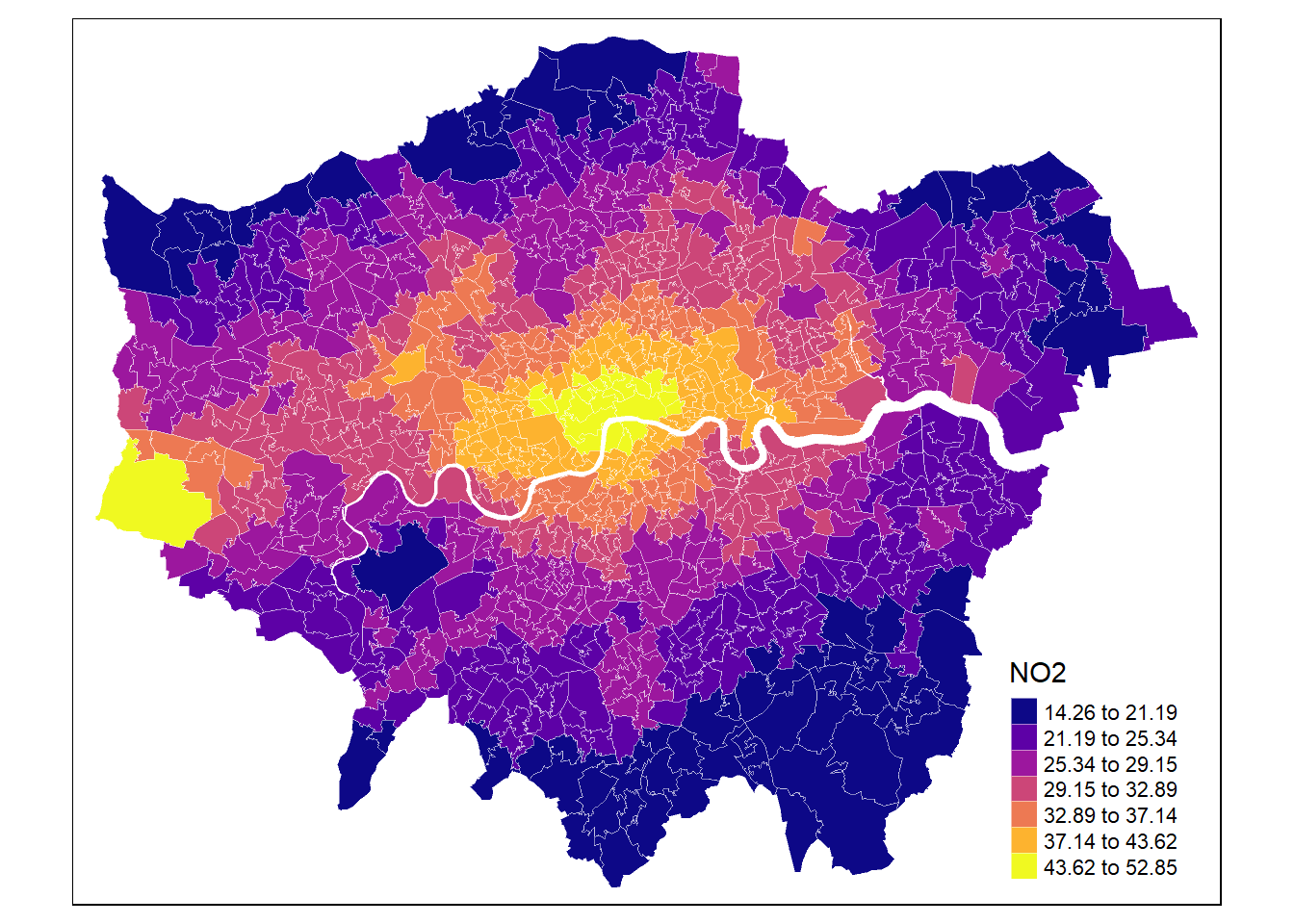

Tmap allows to easily combine different objects by defining a new object via tm_shape().

# Define colours
cols <- viridis(n = 7, direction = 1, option = "C")

mp1 <-  tm_shape(msoa.spdf) + 
  tm_fill(col = "no2", 
          style = "fisher", # algorithm to def cut points
          n = 7, # Number of requested cut points
          palette = cols, # colours
          alpha = 1, # transparency 
          title = "NO2", 
          legend.hist = FALSE # histogram next to map?
          ) +
  tm_borders(col = "white", lwd = 0.5, alpha = 0.5) +
  tm_shape(ulez.spdf) +
  tm_borders(col = "red", lwd = 1, alpha = 1) 

mp1

And it is easy to change the layout.

# Define colours
cols <- viridis(n = 7, direction = 1, option = "C")

mp1 <-  tm_shape(msoa.spdf) + 
  tm_fill(col = "no2", 
          style = "fisher", # algorithm to def cut points
          n = 7, # Number of requested cut points
          palette = cols, # colours
          alpha = 1, # transparency 
          title = expression('in'~mu*'g'/m^{3}), 
          legend.hist = FALSE # histogram next to map?
          ) +
  tm_borders(col = "white", lwd = 0.5, alpha = 0.5) +
  tm_shape(ulez.spdf) +
  tm_borders(col = "red", lwd = 1, alpha = 1) +
  tm_layout(frame = FALSE,
            legend.frame = TRUE, legend.bg.color = TRUE,
            legend.position = c("right", "bottom"),
            legend.outside = FALSE,
            main.title = "NO2", 
            main.title.position = "center",
            main.title.size = 1.6,
            legend.title.size = 0.8,
            legend.text.size = 0.8)

mp1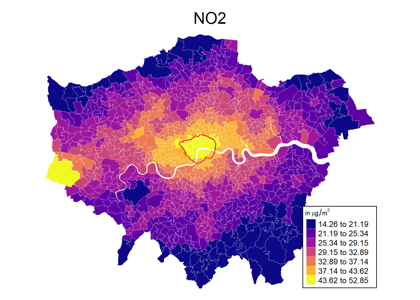

1.5.2 ggplot

For those of you have rather stick with the basic ggplot package, we can also use ggplot for spatial maps.

gp <- ggplot(msoa.spdf)+
    geom_sf(aes(fill = no2))+
    scale_fill_viridis_c(option = "B")+
    coord_sf(datum = NA)+
    theme_map()+
    theme(legend.position = c(.9, .6))
gp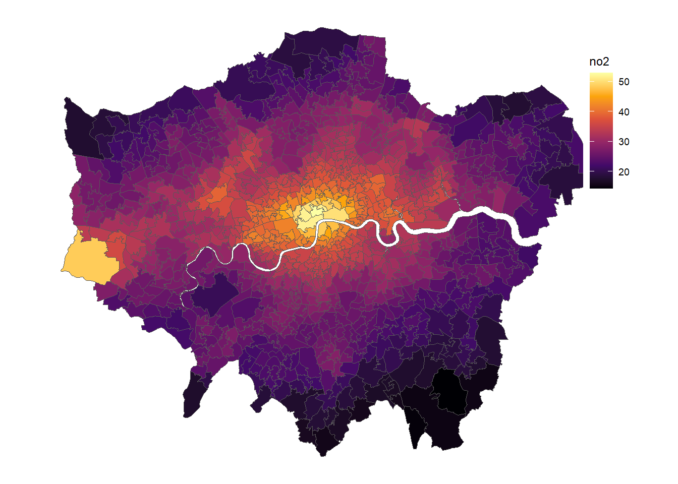

# Get some larger scale boundaries
borough.spdf <- st_read(dsn = paste0("_data", "/statistical-gis-boundaries-london/ESRI"),
                     layer = "London_Borough_Excluding_MHW" # Note: no file ending
                     )

Reading layer `London_Borough_Excluding_MHW' from data source 
  `C:\work\Lehre\Geodata_Spatial_Regression_short\_data\statistical-gis-boundaries-london\ESRI' 
  using driver `ESRI Shapefile'
Simple feature collection with 33 features and 7 fields
Geometry type: MULTIPOLYGON
Dimension:     XY
Bounding box:  xmin: 503568.2 ymin: 155850.8 xmax: 561957.5 ymax: 200933.9
Projected CRS: OSGB36 / British National Grid

# transform to only inner lines
borough_inner <- ms_innerlines(borough.spdf)

# Plot with inner lines
gp <- ggplot(msoa.spdf)+
    geom_sf(aes(fill = no2), color = NA)+
    scale_fill_viridis_c(option = "A")+
    geom_sf(data = borough_inner, color = "gray92")+
    geom_sf(data = ulez.spdf, color = "red", fill = NA)+
    coord_sf(datum = NA)+
    theme_map()+
    labs(fill = "NO2")+
    theme(legend.position = c(.9, .6))
gp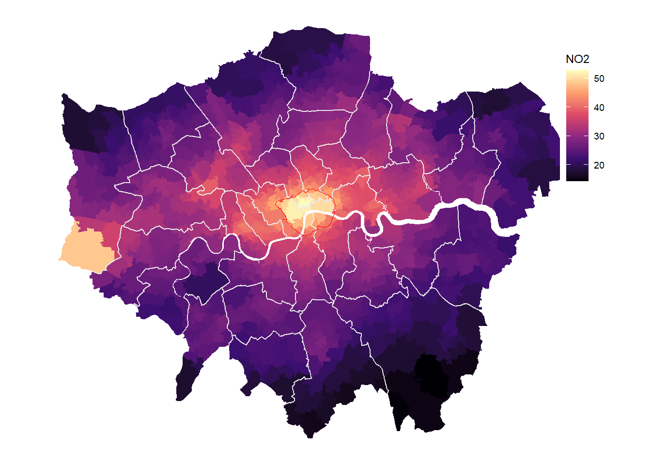

1.6 Exercise

1. What is the difference between a spatial “sf” object and a conventional “data.frame”? What’s the purpose of the function st_drop_geometry()?

It’s the same. A spatial “sf” object just has an additional column containing the spatial coordinates.

2. Using msoa.spdf, please create a spatial data frame that contains only the MSOA areas that are within the ulez zone.

sub4.spdf <- msoa.spdf[ulez.spdf, ]

3. Please create a map for London (or only the msoa-ulez subset) which shows the share of Asian residents (or any other ethnic group).

gp <- ggplot(msoa.spdf)+
    geom_sf(aes(fill = per_asian))+
    scale_fill_viridis_c(option = "E")+
    coord_sf(datum = NA)+
    theme_map()+
    theme(legend.position = c(.9, .6))
gp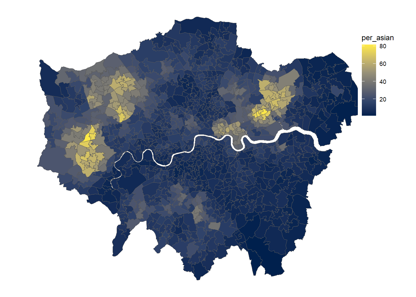

4. Please calculate the distance of each MSOA to the London city centre

1. use google maps to get lon and lat,
2. use st_as_sf() to create the spatial point
3. use st_distance() to calculate the distance

### Distance to city center
# Define centre
centre <- st_as_sf(data.frame(lon = -0.128120855701165, 
                              lat = 51.50725909644806),
                   coords = c("lon", "lat"), 
                   crs = 4326)
# Reproject
centre <- st_transform(centre, crs = st_crs(msoa.spdf))
# Calculate distance
msoa.spdf$dist_centre <- as.numeric(st_distance(msoa.spdf, centre)) / 1000
# hist(msoa.spdf$dist_centre)

5. Can you create a plot with the distance to the city centre and pub counts next to each other?

# Define colours
cols <- viridis(n = 10, direction = 1, option = "B")
cols2 <- viridis(n = 10, direction = 1, option = "E")


mp1 <-  tm_shape(msoa.spdf) + 
  tm_fill(col = "dist_centre", 
          style = "fisher", # algorithm to def cut points
          n = 10, # Number of requested cut points
          palette = cols, # colours
          alpha = 1, # transparency 
          title = "Distance", 
          legend.hist = FALSE # histogram next to map?
          ) +
  tm_borders(col = "white", lwd = 0.5, alpha = 0.5) +
  tm_layout(frame = FALSE,
            legend.frame = TRUE, legend.bg.color = TRUE,
            legend.position = c("right", "bottom"),
            legend.outside = FALSE,
            main.title = "Dist centre", 
            main.title.position = "center",
            main.title.size = 1.6,
            legend.title.size = 0.8,
            legend.text.size = 0.8)


mp2 <-  tm_shape(msoa.spdf) + 
  tm_fill(col = "dist_centre", 
          style = "quantile", # algorithm to def cut points
          n = 10, # Number of requested cut points
          palette = cols, # colours
          alpha = 1, # transparency 
          title = "Distance", 
          legend.hist = FALSE # histogram next to map?
          ) +
  tm_borders(col = "white", lwd = 0.5, alpha = 0.5) +
  tm_layout(frame = FALSE,
            legend.frame = TRUE, legend.bg.color = TRUE,
            legend.position = c("right", "bottom"),
            legend.outside = FALSE,
            main.title = "Dist centre", 
            main.title.position = "center",
            main.title.size = 1.6,
            legend.title.size = 0.8,
            legend.text.size = 0.8)


mp3 <-  tm_shape(msoa.spdf) + 
  tm_fill(col = "pubs_count", 
          style = "fisher", # algorithm to def cut points
          n = 10, # Number of requested cut points
          palette = cols, # colours
          alpha = 1, # transparency 
          title = "Count", 
          legend.hist = FALSE # histogram next to map?
          ) +
  tm_borders(col = "white", lwd = 0.5, alpha = 0.5) +
  tm_layout(frame = FALSE,
            legend.frame = TRUE, legend.bg.color = TRUE,
            legend.position = c("right", "bottom"),
            legend.outside = FALSE,
            main.title = "Pubs", 
            main.title.position = "center",
            main.title.size = 1.6,
            legend.title.size = 0.8,
            legend.text.size = 0.8)


mp4 <-  tm_shape(msoa.spdf) + 
  tm_fill(col = "pubs_count", 
          style = "quantile", # algorithm to def cut points
          n = 10, # Number of requested cut points
          palette = cols, # colours
          alpha = 1, # transparency 
          title = "Count", 
          legend.hist = FALSE # histogram next to map?
          ) +
  tm_borders(col = "white", lwd = 0.5, alpha = 0.5) +
  tm_layout(frame = FALSE,
            legend.frame = TRUE, legend.bg.color = TRUE,
            legend.position = c("right", "bottom"),
            legend.outside = FALSE,
            main.title = "Pubs", 
            main.title.position = "center",
            main.title.size = 1.6,
            legend.title.size = 0.8,
            legend.text.size = 0.8)


tmap_arrange(mp1, mp2, mp3, mp4, ncol = 2, nrow = 2)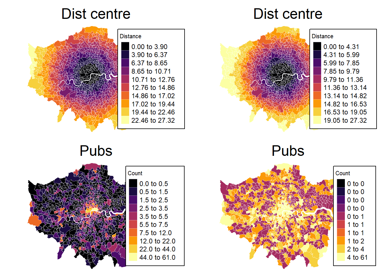

1.6.1 Geogrphic cter

# Make one single schape
london <- st_union(msoa.spdf)

# Calculate center
cent <- st_centroid(london)

mapview(cent)

Lee, Barrett A., Sean F. Reardon, Glenn Firebaugh, Chad R. Farrell, Stephen A. Matthews, and David O’Sullivan. 2008. “Beyond the Census Tract: Patterns and Determinants of Racial Segregation at Multiple Geographic Scales.” American Sociological Review 73 (5): 766–91. https://doi.org/10.1177/000312240807300504.

Lovelace, Robin, Jakub Nowosad, and Jannes Muenchow. 2019. Geocomputation with R. 1st ed. Chapman & Hall/CRC the R Series. Boca Raton: Chapman & Hall/CRC.

Mohai, Paul, and Robin Saha. 2007. “Racial Inequality in the Distribution of Hazardous Waste: A National-Level Reassessment.” Social Problems 54 (3): 343–70. https://doi.org/10.1525/sp.2007.54.3.343.