Impact evaluation using secondary data
2023-11-15
What IS Causation?
- \(X\) causes \(Y\) if we can intervene and change \(X\) without changing anything else, and \(Y\) changes
- \(Y\) “listens to” \(X\)
- \(X\) may not be the only thing that causes \(Y\)!

What IS Causation?
- \(X\) causes \(Y\) if we can intervene and change \(X\) without changing anything else, and \(Y\) changes
- \(Y\) “listens to” \(X\)
- \(X\) may not be the only thing that causes \(Y\)!
Drawing a DAG
Consider all the variables likely to be important to the data-generating process (including variables we can’t observe!)
For simplicity, combine some similar ones together or prune those that aren’t very important
Consider which variables are likely to affect others, and draw arrows connecting them
Test some testable implications of the model (to see if we have a correct one!)
Drawing a DAG
Drawing an arrow requires a direction - making a statement about causality!
Omitting an arrow makes an equally important statement too!
- In fact, we will need omitted arrows to show causality!
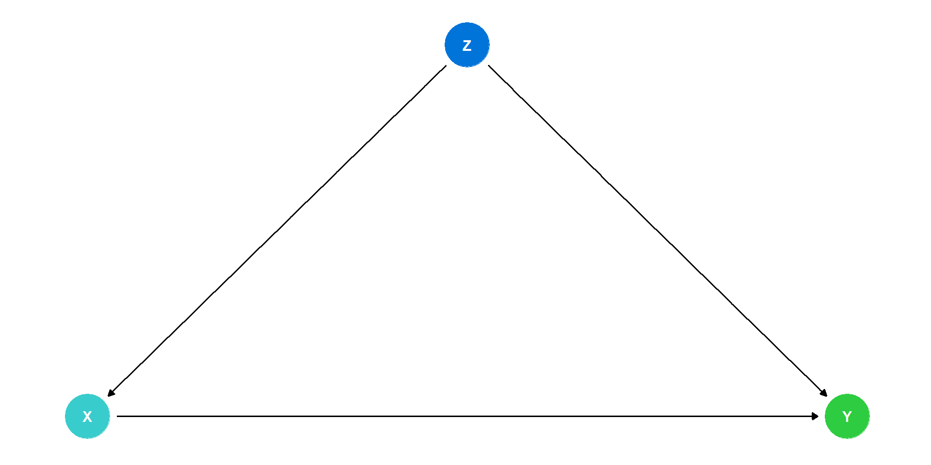
If two variables are correlated, but neither causes the other, likely they are both caused by another (perhaps unobserved) variable - add it!
There should be no cycles or loops (if so, there’s probably another missing variable, such as time)
DAG Example I

DAG Example I
- What other variables are important?
- Ability
- Socioeconomic status
- Demographics
- Gravity
- Year of birth
- Location
- Schooling laws
- Job network
DAG Example I
In social science and complex systems, 1000s of variables could plausibly be in the DAG!
So simplify:
- Ignore trivial things (like gravity)
- Combine similar variables (Socioeconomic status, Demographics, Location) if not interesting per se \(\rightarrow\) Background

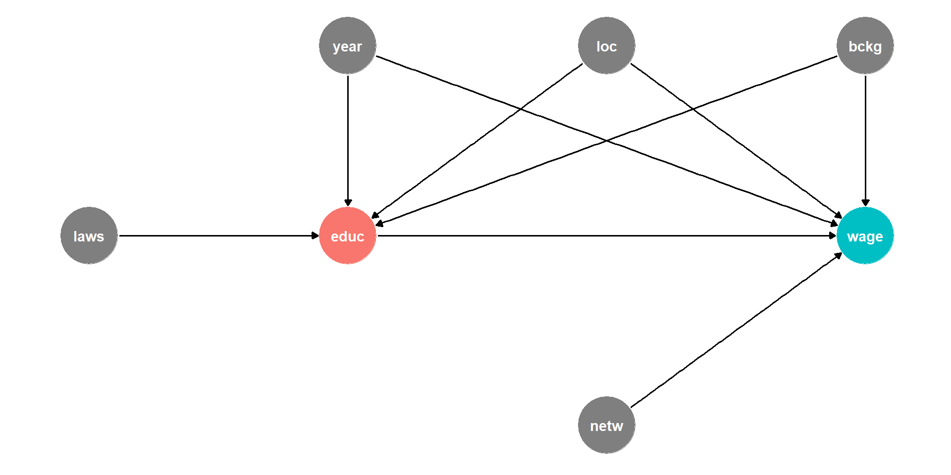
DAG Example II
Background, Year of birth, Location, Compulsory schooling, all cause education
Background, year of birth, location, job networks probably cause wages
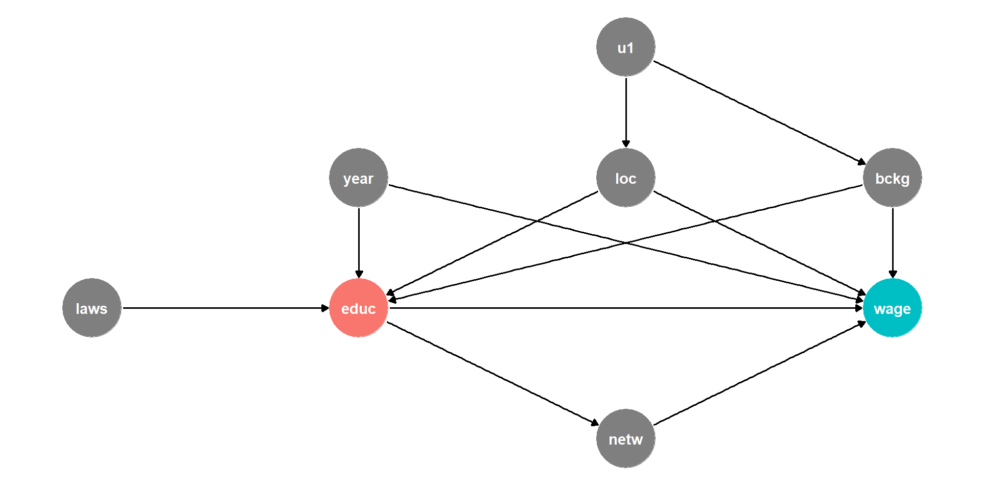
DAG Example II
Background, Year of birth, Location, Compulsory schooling, all cause education
Background, year of birth, location, job networks probably cause wages
Job networks in fact is probably caused by education!
Location and background probably both caused by unobserved factor (
u1)

DAG Example II
This is messy, but we have a causal model!
Makes our assumptions explicit, and many of them are testable
DAG suggests certain relationships that will not exist:
- all relationships between
lawsandnetwgo througheduc - so if we controlled for
educ, thencor(laws,netw)should be zero!
- all relationships between
Potential outcomes, counterfactuals, and the road not taken
The problem of confounding
Naive comparison of treated vs untreated is often biased
- Individuals select themselves into a treatment group, causing a bias.
- Some unobserved characteristics causes treatment and outcome, making the observed relationship spurious.

The problem of confounding
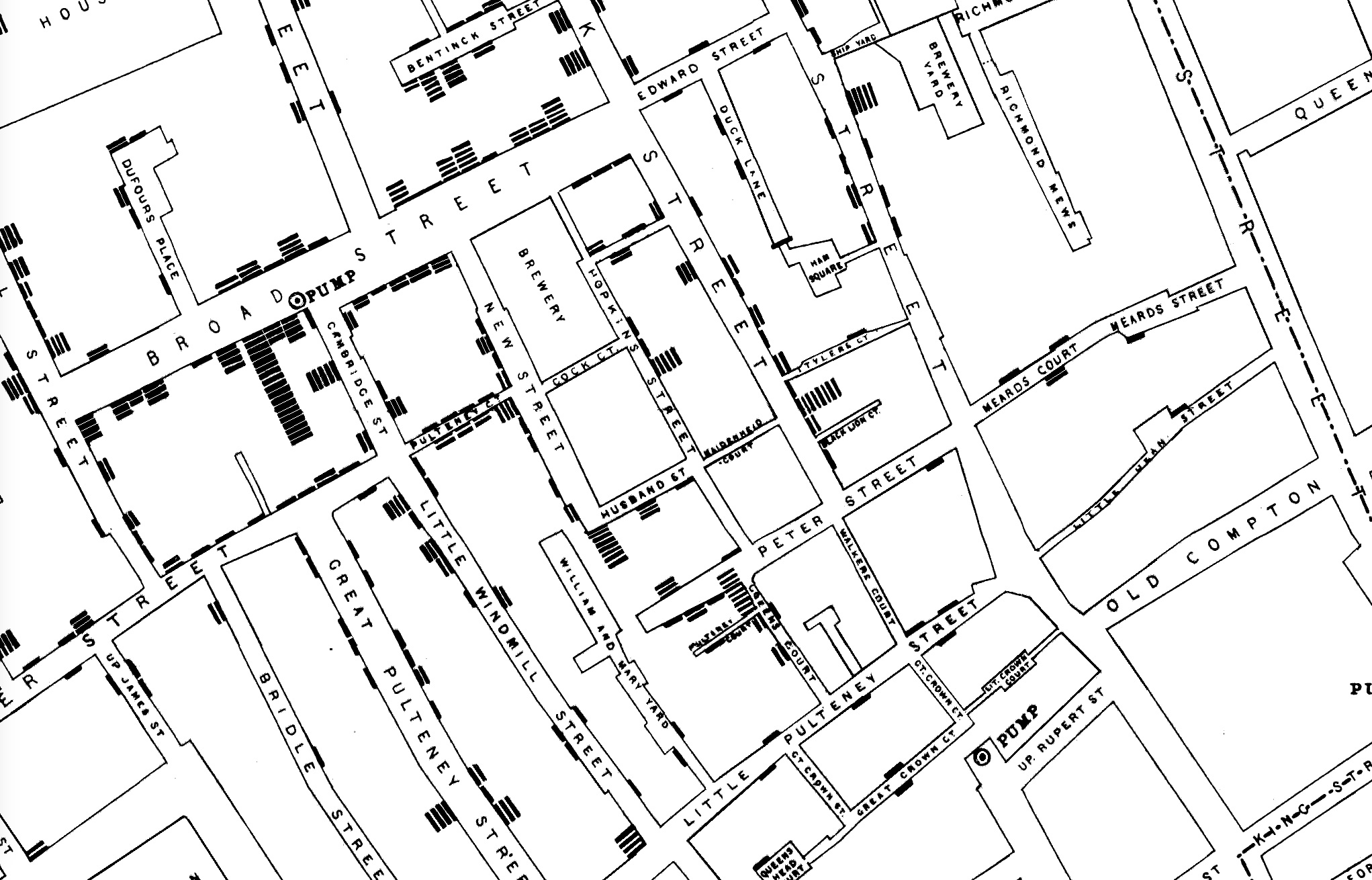
John Snow and Cholera: Youtube
The beauty of randomisation
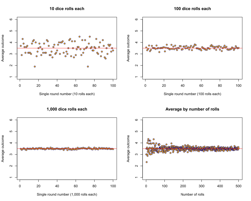
Law of large numbers
- if we randomly assign treatment
- and \(N\) is sufficiently large
- treatment and control group should be identical on average
- each group should have the same mean as the population
- that applies to all their characteristics (e.g. gender, age, motivation, political views…)
Randomised Control Trials

Example: Peer-group intervention
Carrell, Sacerdote, and West (2013)
- United States Air Force Academy
- Students randomly assigned to peer groups
- Positive peer effect on academic performance
New experiment of policy instrument
- Assignment to “optimally” designed peer groups
- “Optimal” policy has negative effect on performance
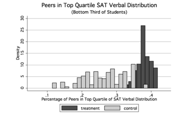
“These results illustrate how policies that manipulate peer groups for a desired social outcome can be confounded by changes in the endogenous patterns of social interactions within the group.”
IV: The problem
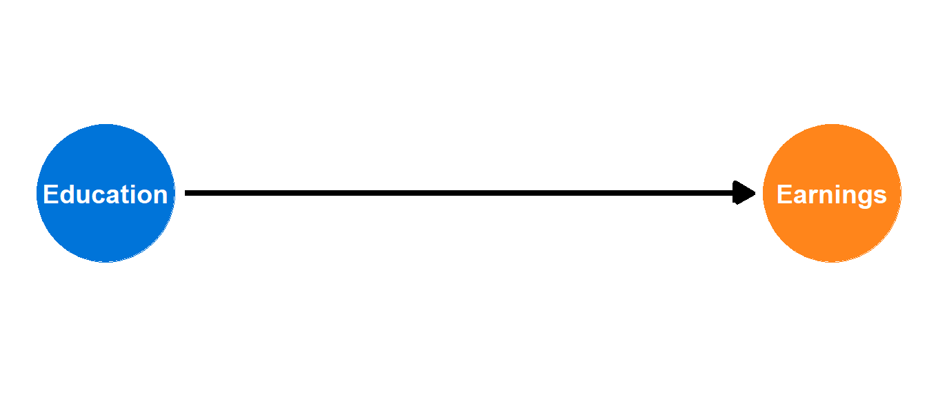
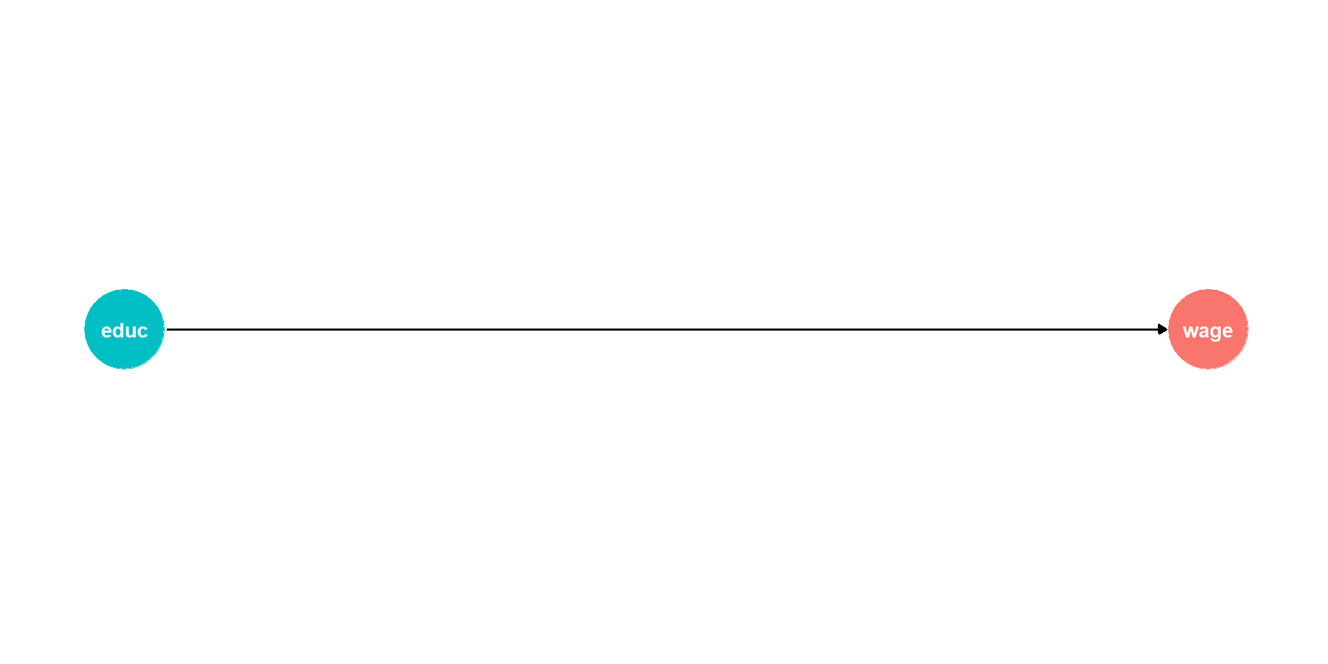
\[\color{#FF851B}{\text{Earnings}_i} = \beta_0 + \beta_1 \color{#0074D9}{\text{Education}_i} + \varepsilon_i\]
If we ran this regression, would \(\beta_1\) give us the causal effect of education?
No!
- Omitted variable bias!
- Endogeneity!
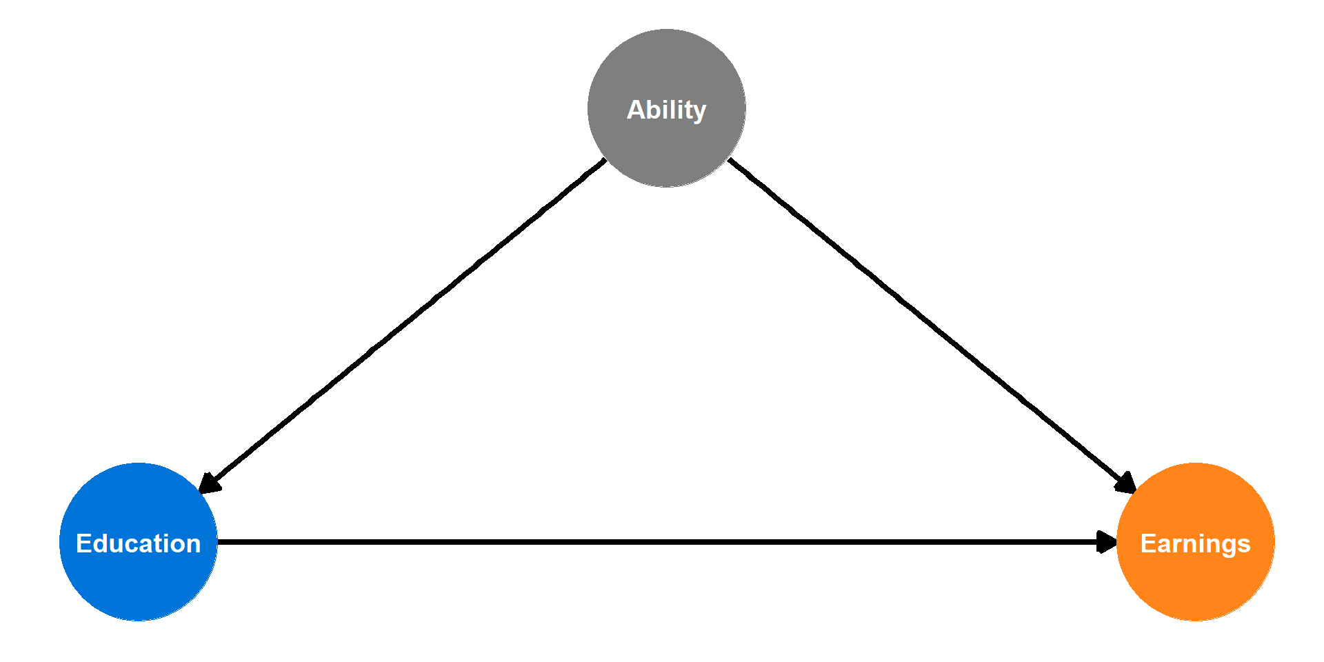
IV: The problem
Exogenous variables
- Value is not determined by anything else in the model
- In a DAG, a node that doesn’t have arrows coming into it
Endogenous variables
- Value is determined by something else in the model
- In a DAG, a node that has arrows coming into it
What is an instrument?
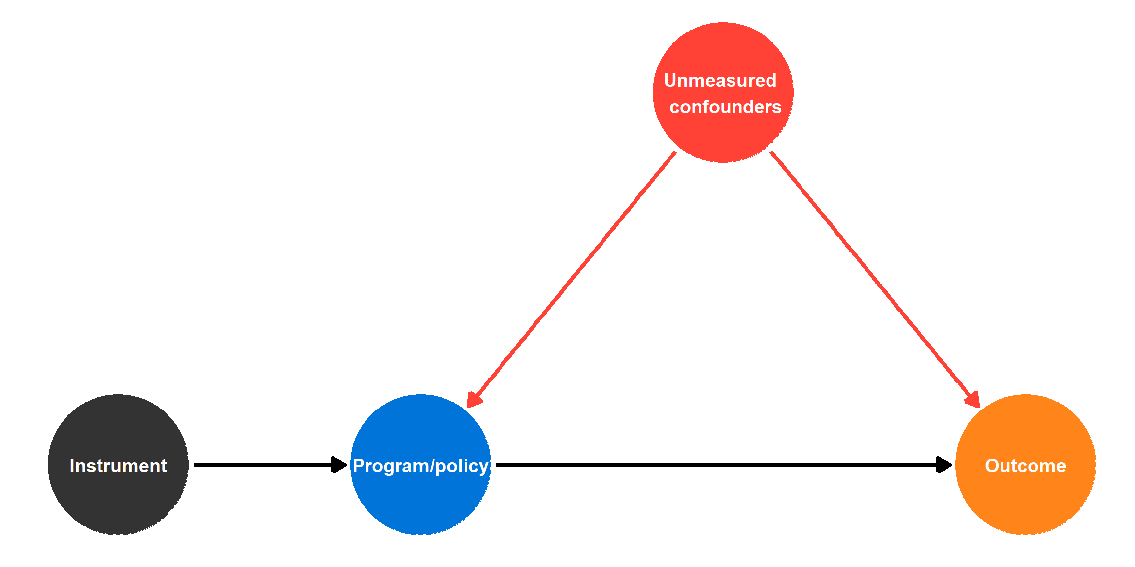
Example of instrument

IV example: Family size and education
First stage: Instrument \(\rightarrow\) Family size
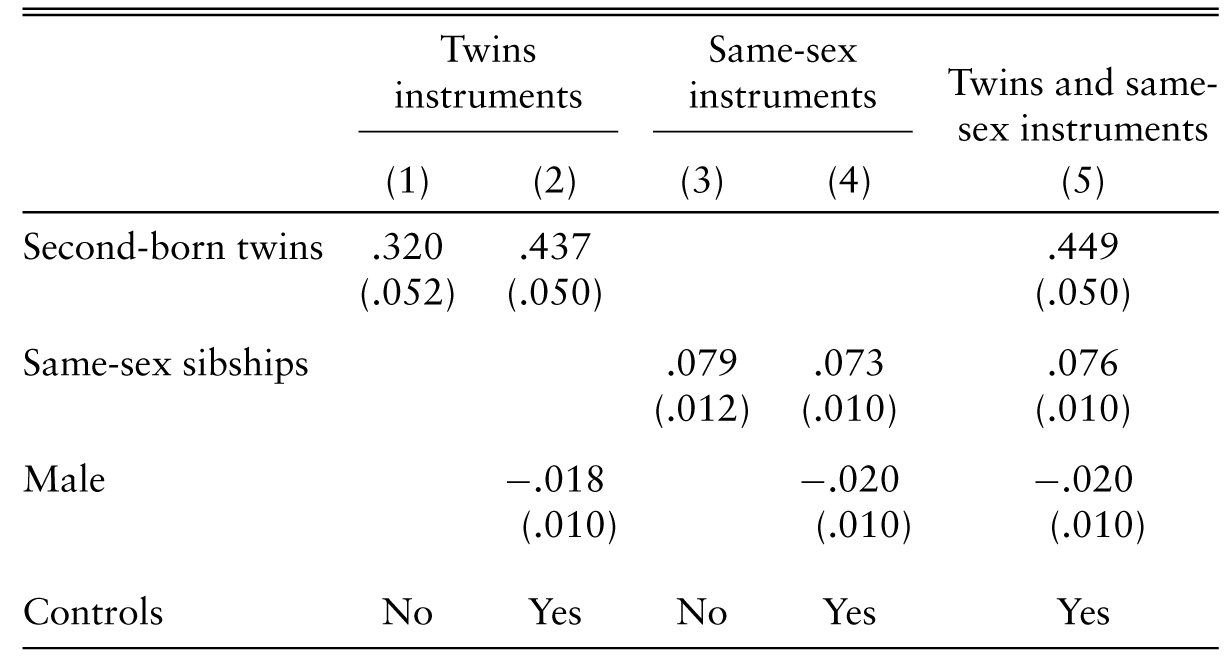
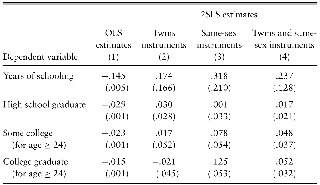
IV example: Family size and education
Second stage: Predicted Family size \(\rightarrow\) Educ
Instruments are hard to find!
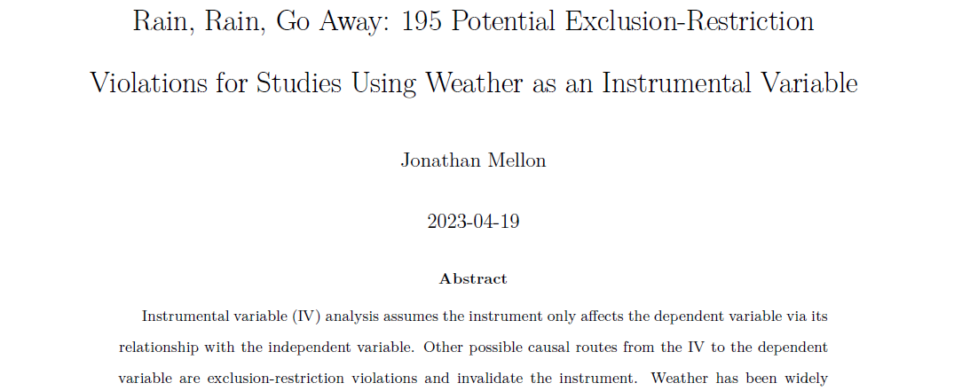
\(\color{red}{\text{Exlusion restriction}}\)
- Instrument causes the outcome only through the policy
- For instance, rainfall is not a good instrument instrument (Mellon 2020)
RDD: Hypothetical example
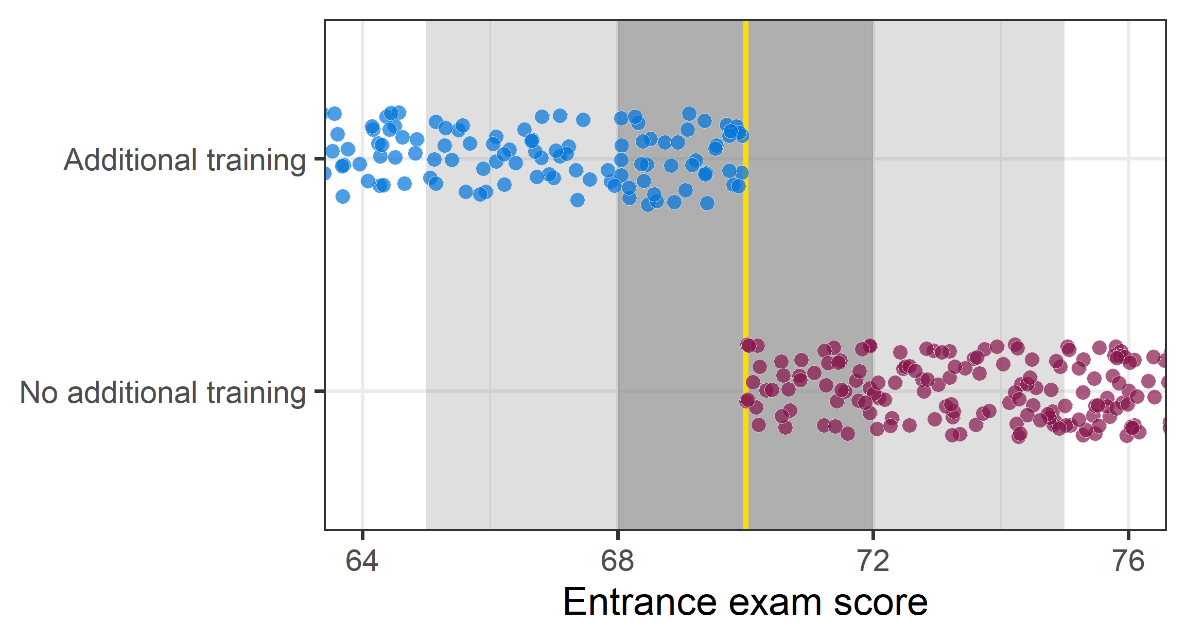
Imagine: An entrance exam and those who score 70 or lower get additional training.
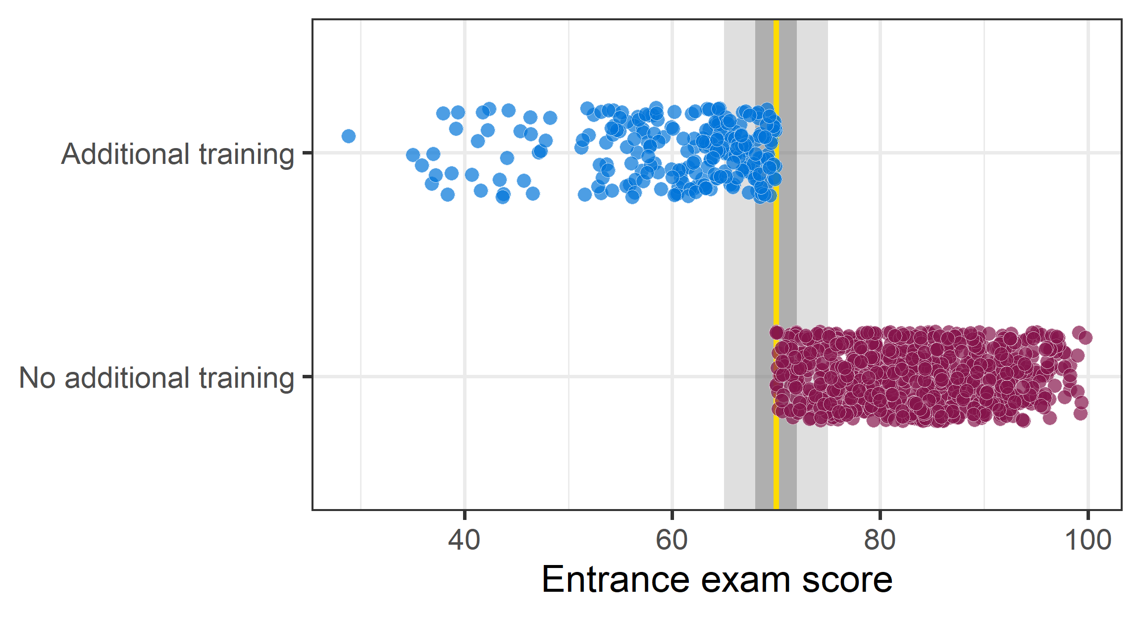
RDD: Hypothetical example
Imagine: A entrance exam and those who score 70 or lower get additional training.
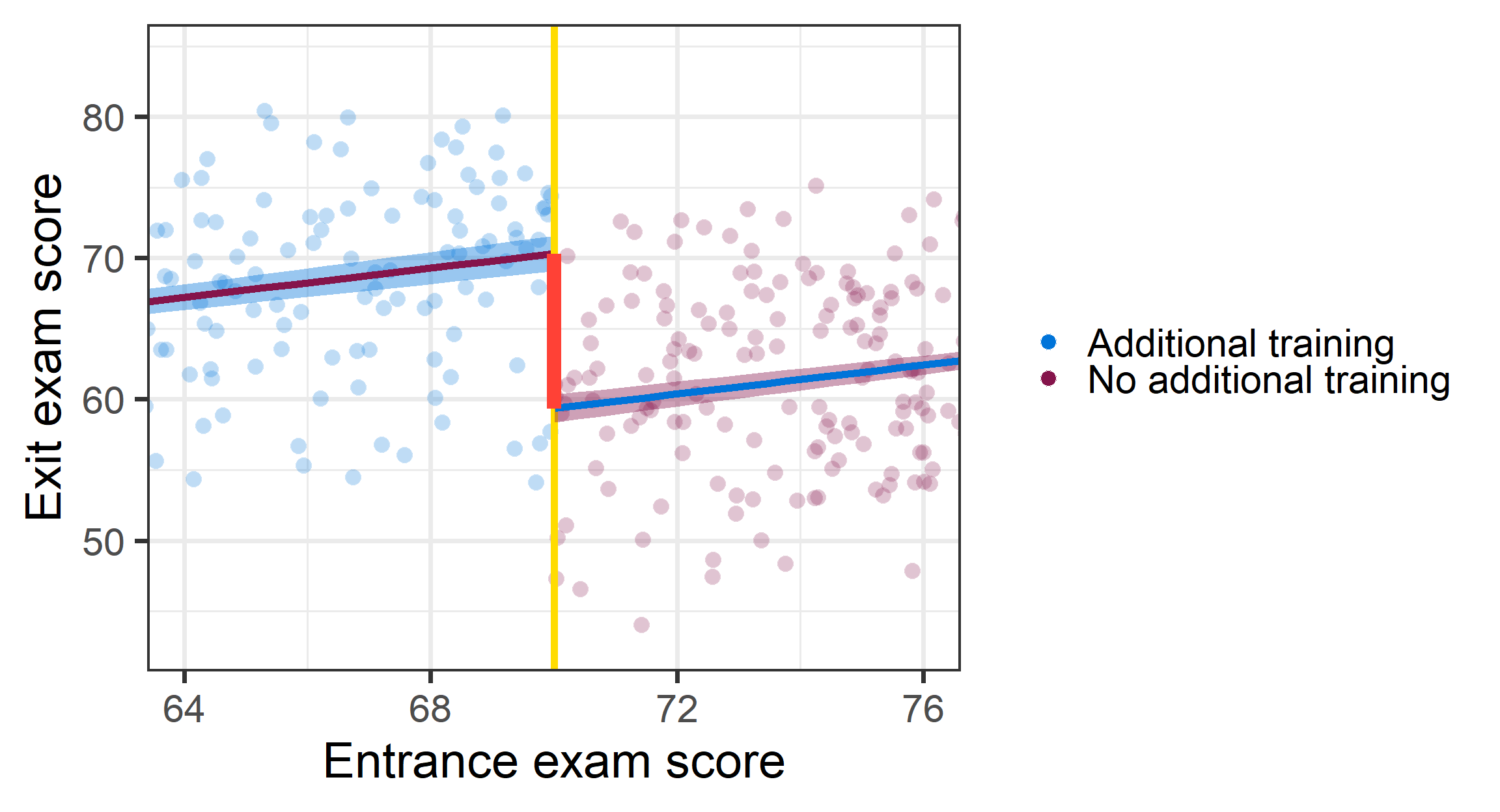
RDD: Hypothetical estimate
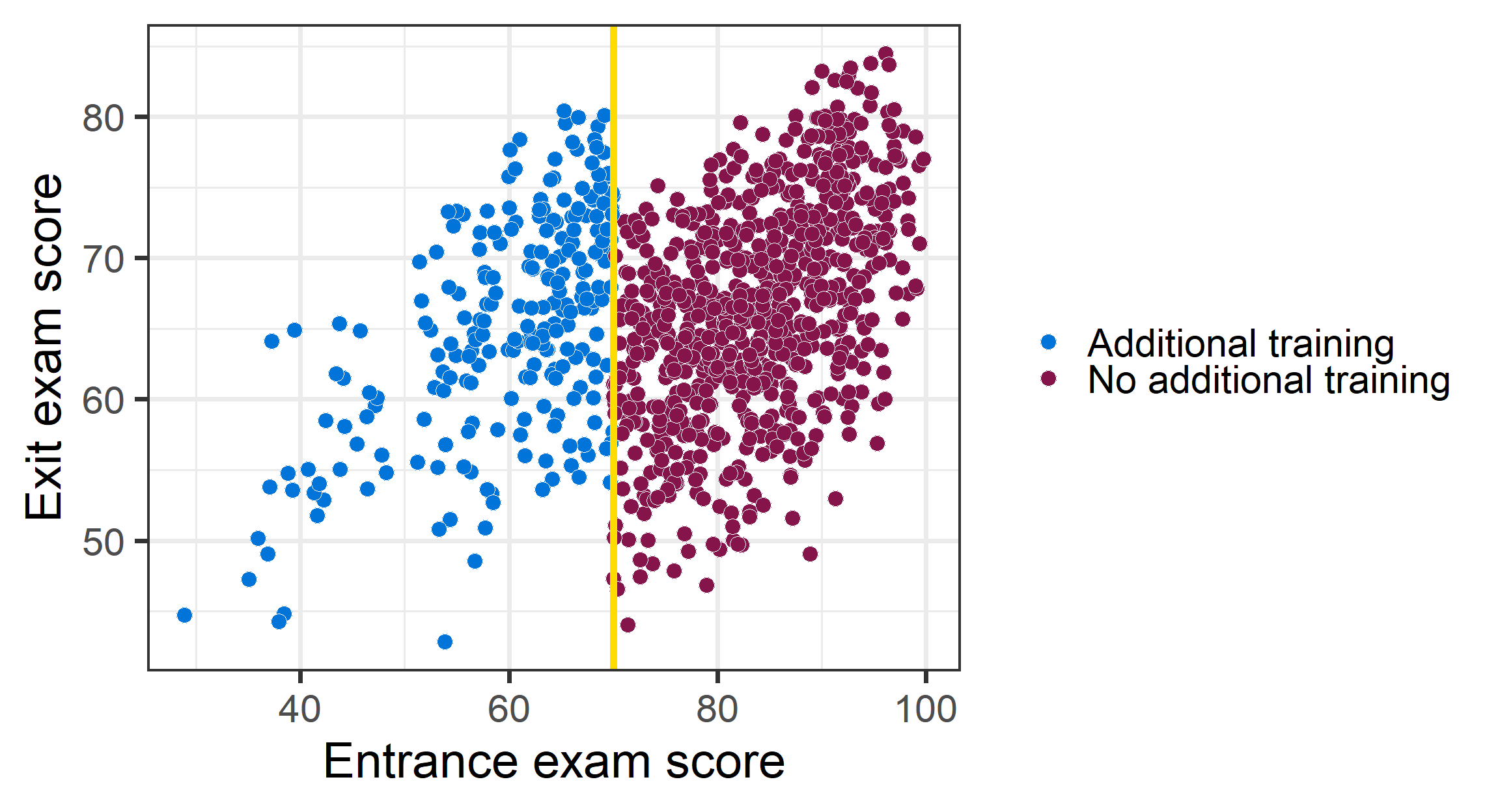
RDD: Hypothetical estimate
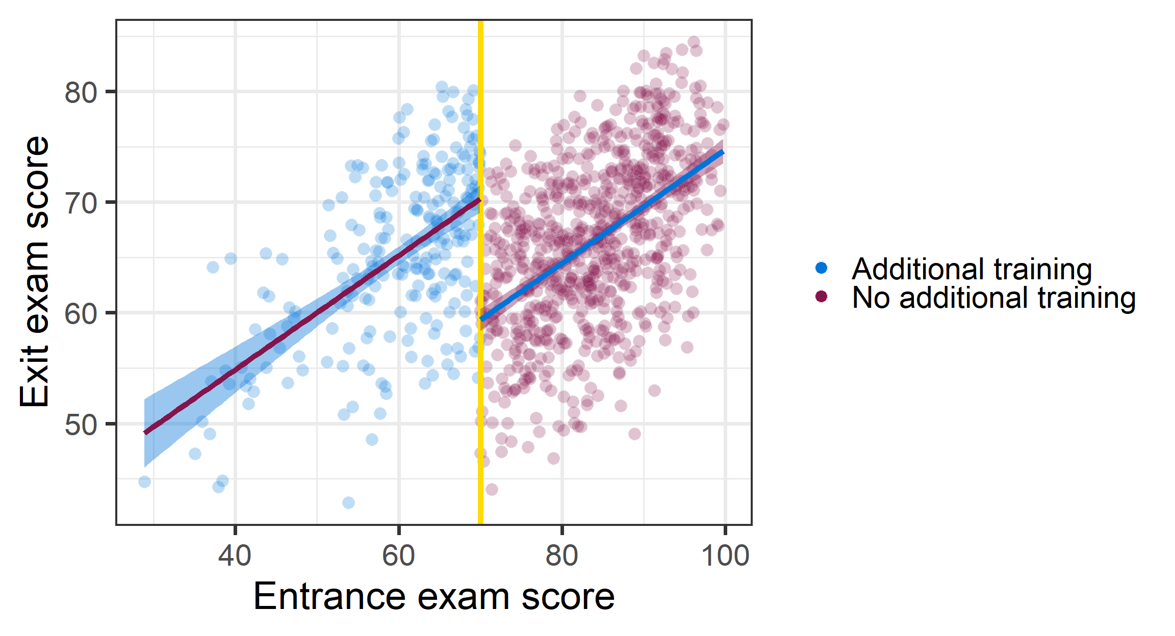
RDD: Hypothetical estimate
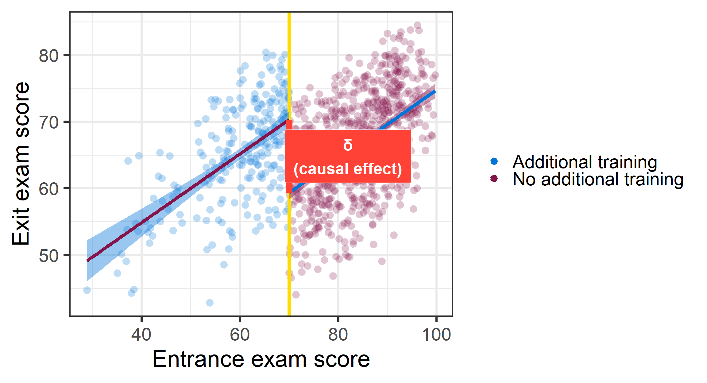
RDD: Hypothetical estimate
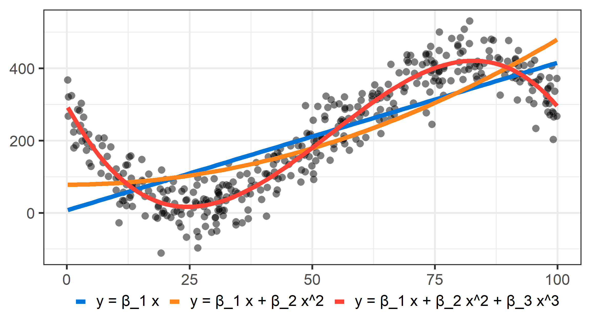
RDD: Drawing lines
Check higher order polynomials!
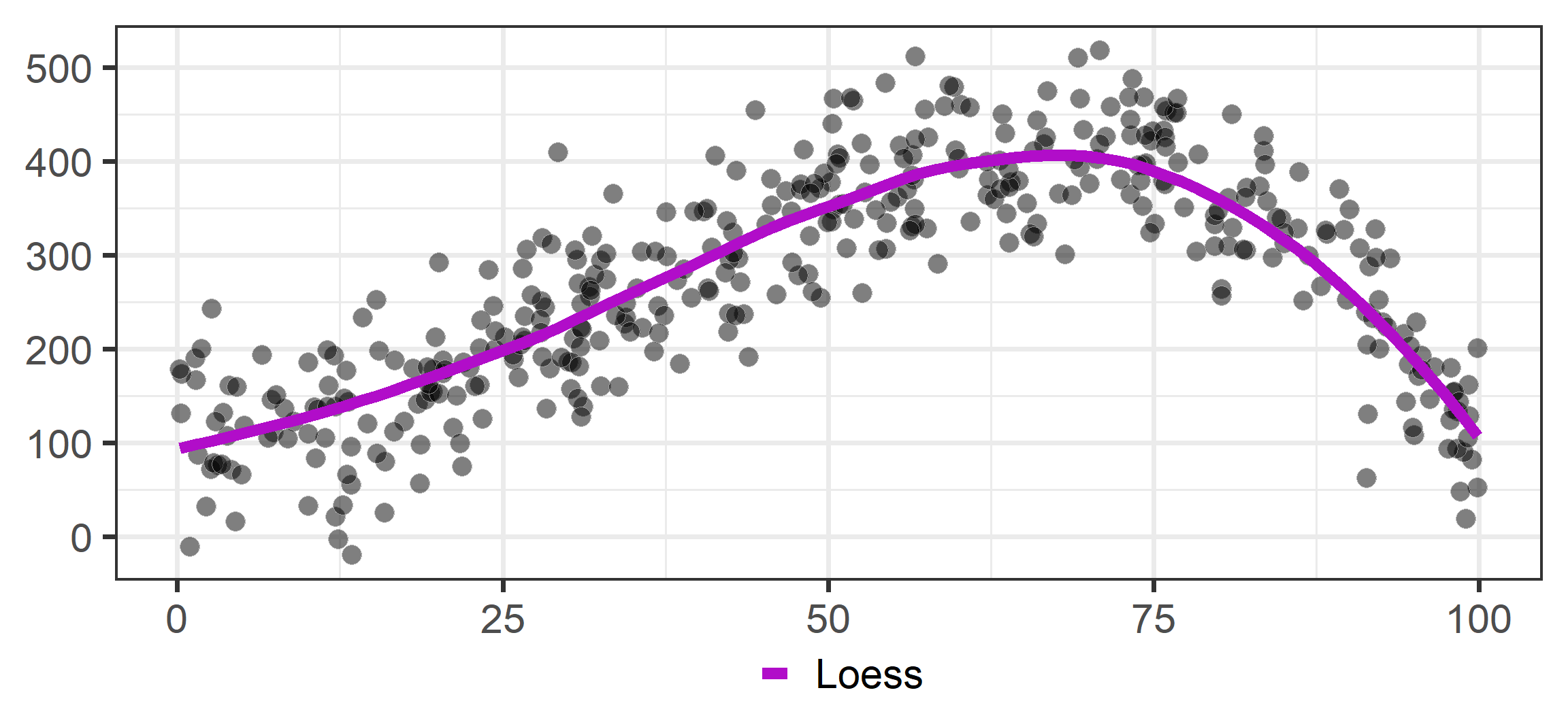
RDD: Drawing lines
Non-parametric methods like LOESS (Locally estimated scatterplot smoothing)
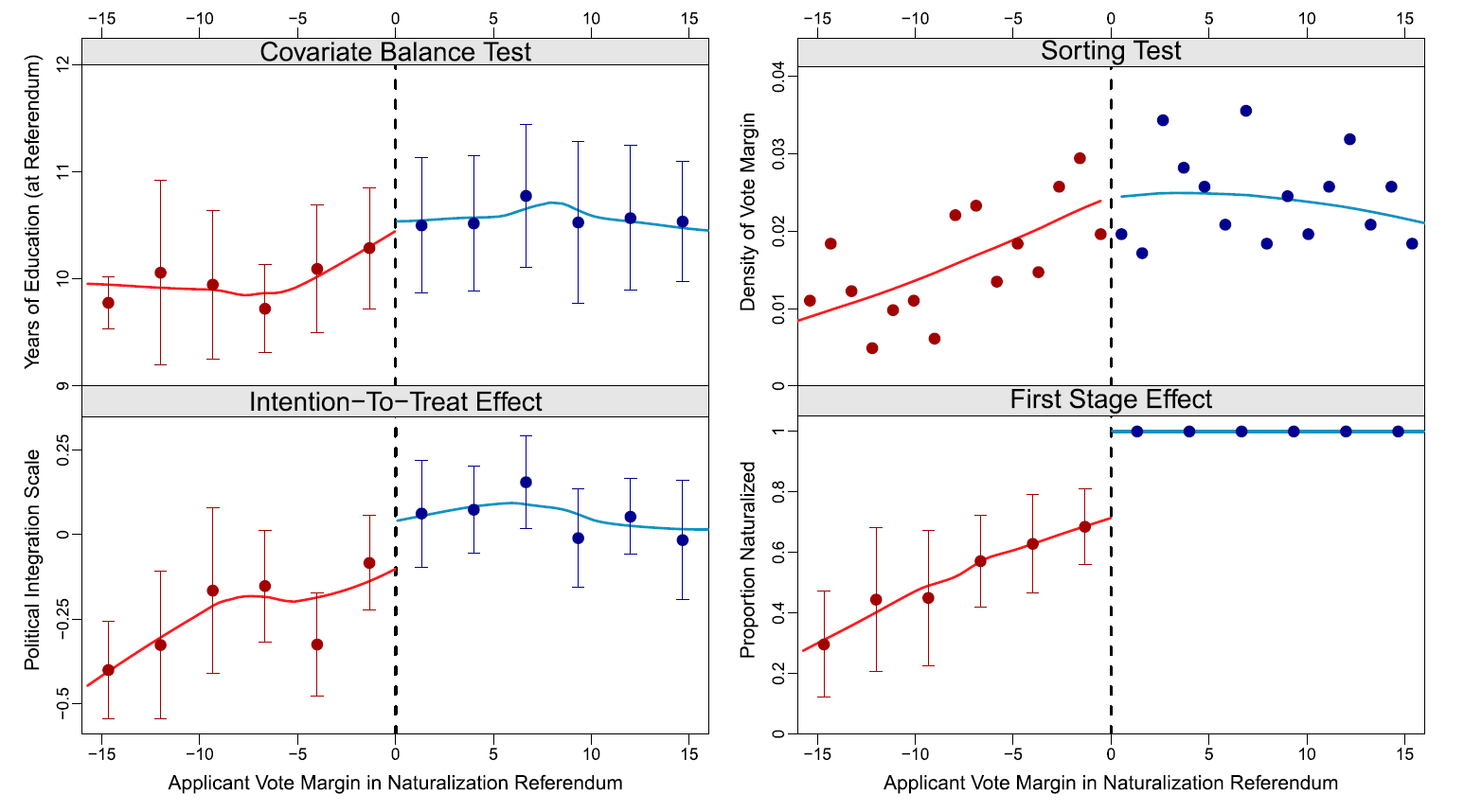
RDD: Naturalisation & Political integration
Hainmueller, Hangartner, and Pietrantuono (2015):
- Switzerland, where some municipalities used referendums as the mechanism to decide naturalization requests
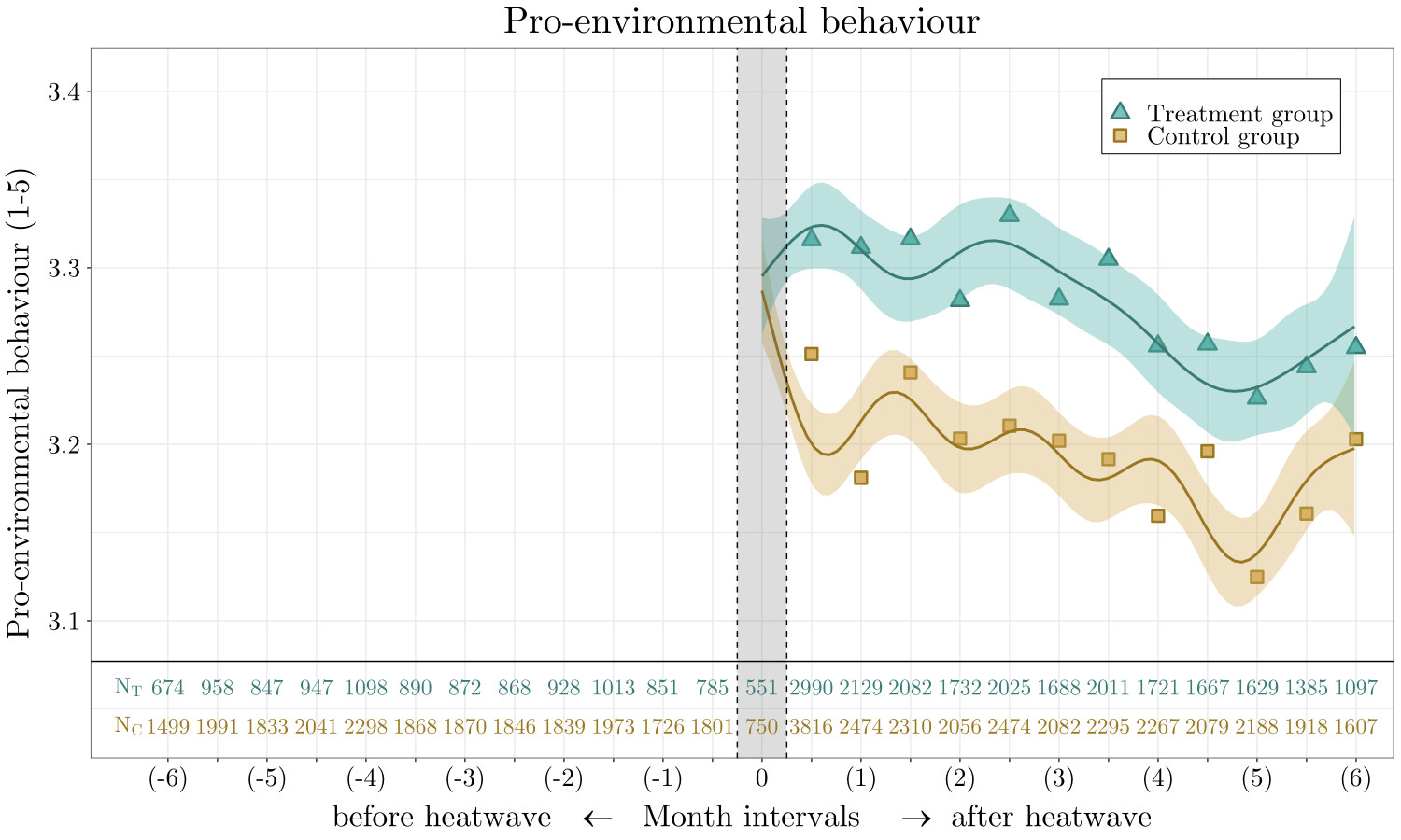
Heatwave exposure & pro-environmental behaviour
Rüttenauer (2023)
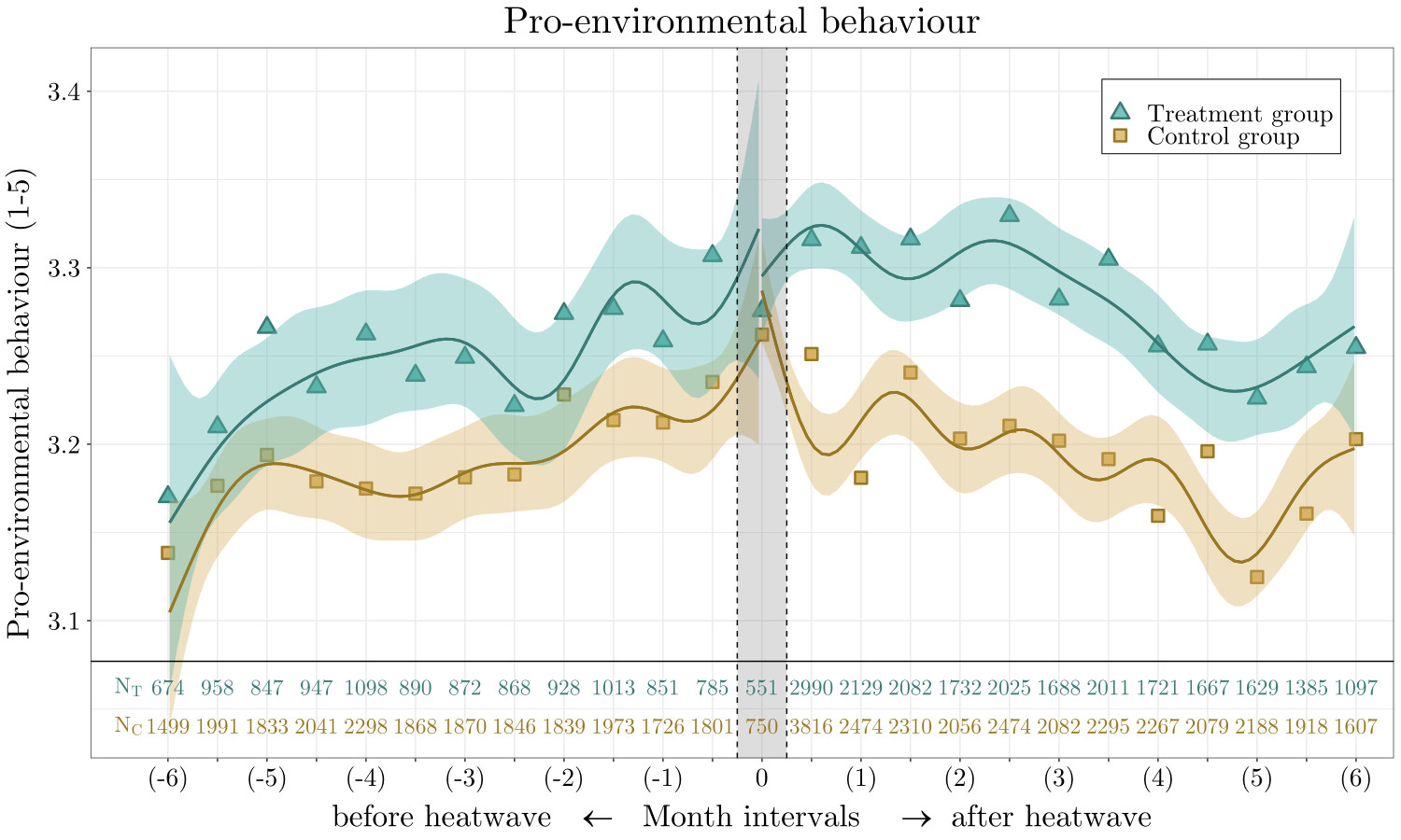
Heatwave exposure & pro-environmental behaviour
Rüttenauer (2023)
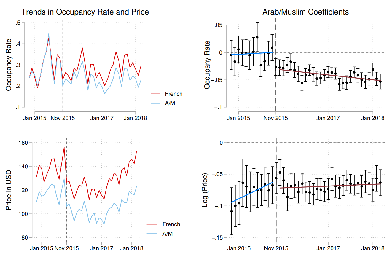
Paris terror attack and discrimination on AirBnB
Wagner and Petev (2019)
DiD: Problems
Comparing only treatment/control
- You’re only looking at post-treatment values
- Impossible to know if change happened because of natural growth
Comparing only before/after
- You’re only looking at the treatment group!
- Impossible to know if change happened because of treatment or just naturally
Simple DiD setup
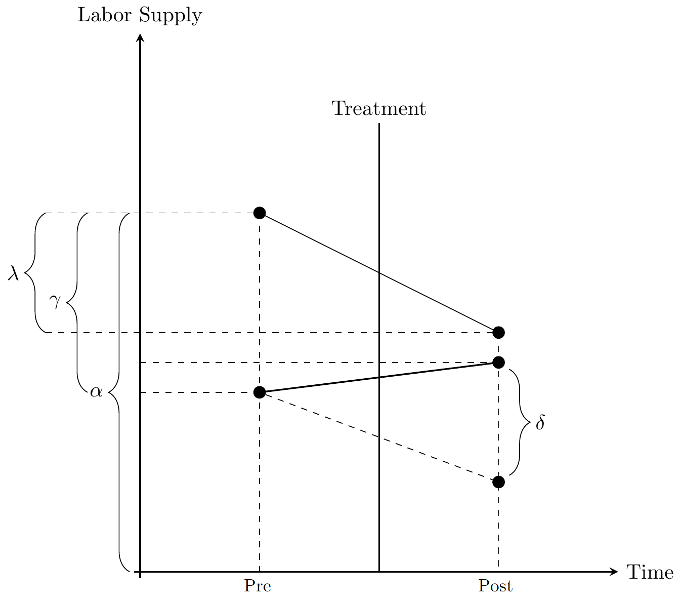
Important:
Monetary Intervention & Banking Panics
Richardson and Troost (2009)
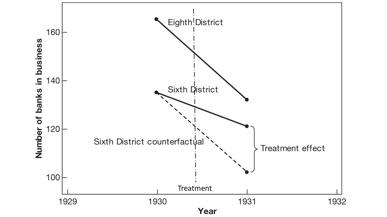
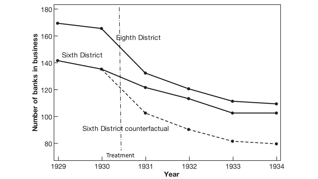
Monetary Intervention & Banking Panics
Parallel trends?
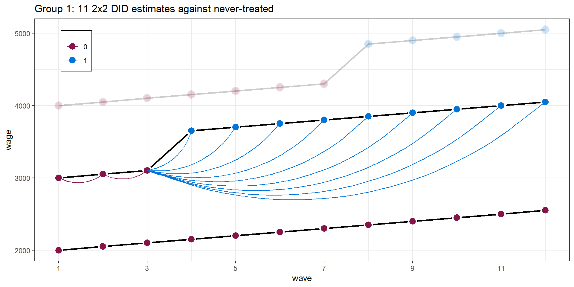
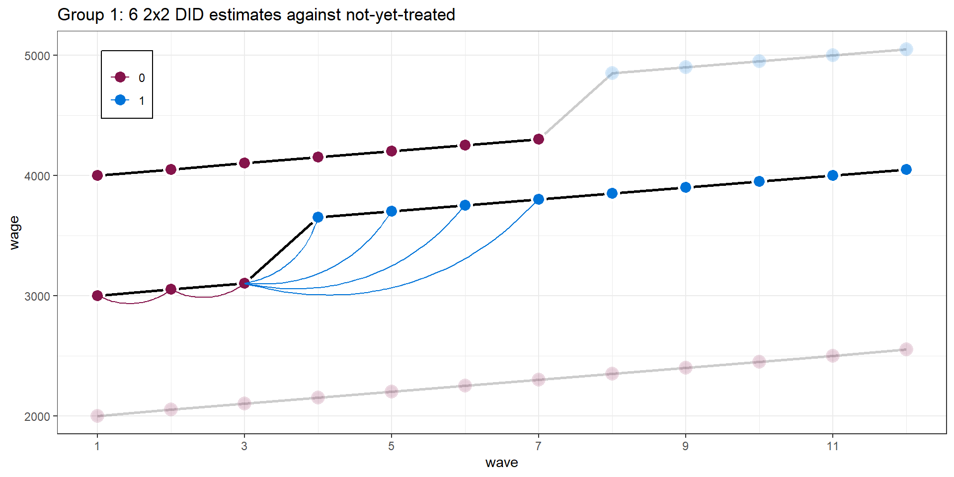
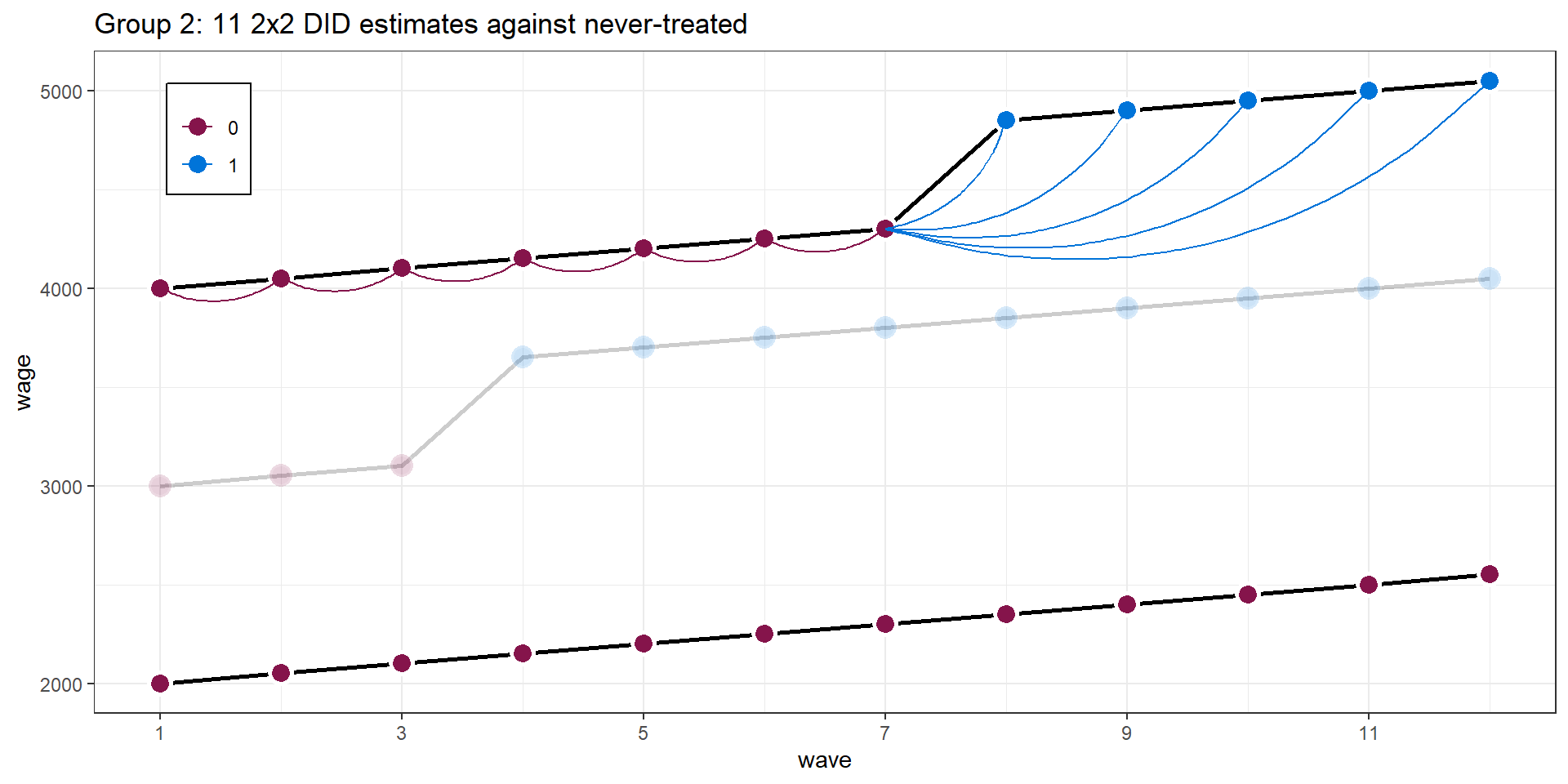
Two-ways FE with multiple treatment periods
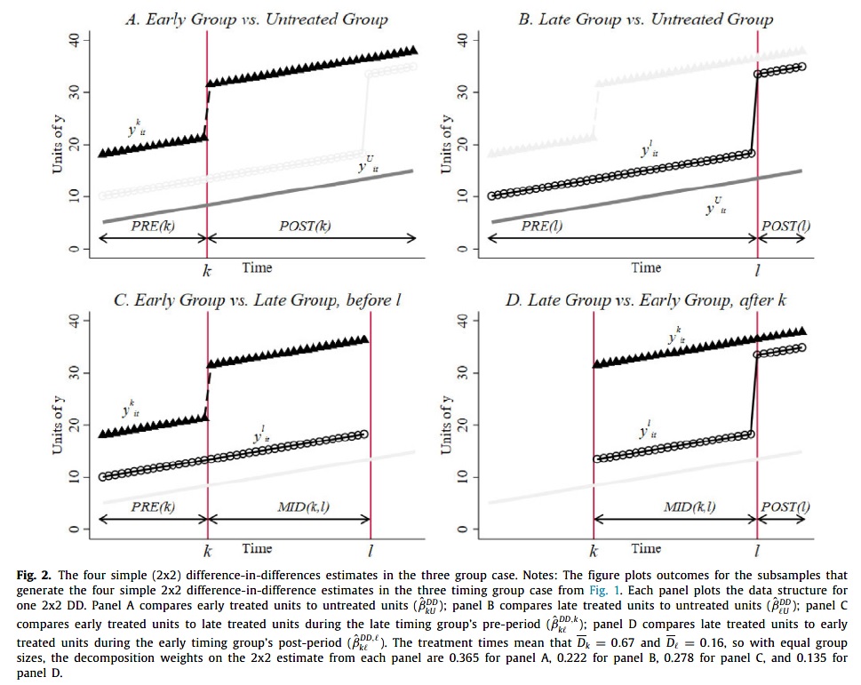
Figure from Goodman-Bacon (2021)
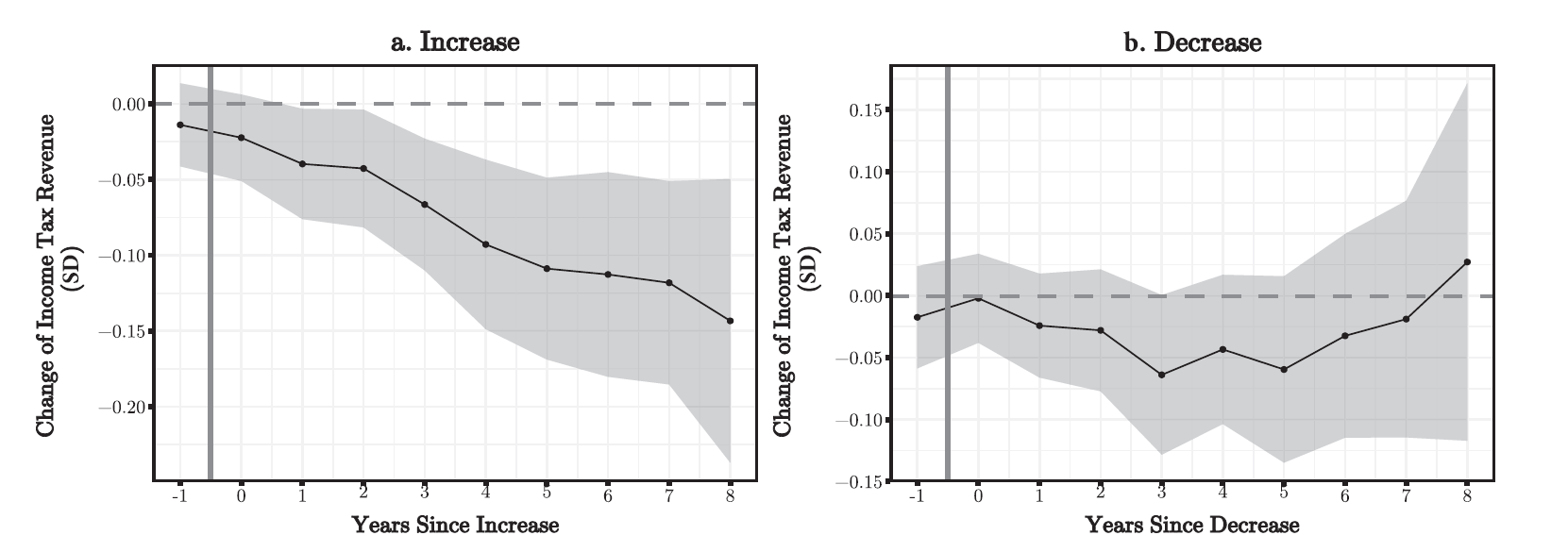
Event Study Design
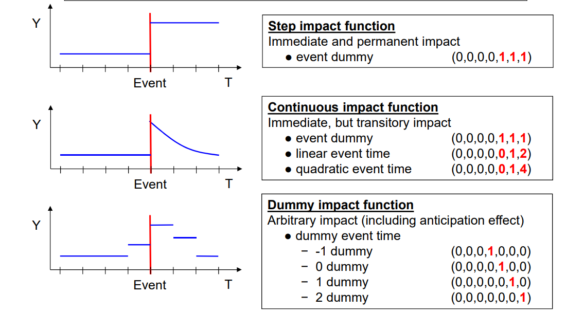
Dynamic Diff-in-Diff
Industrial plant openings & resident’s income
Rüttenauer and Best (2021)
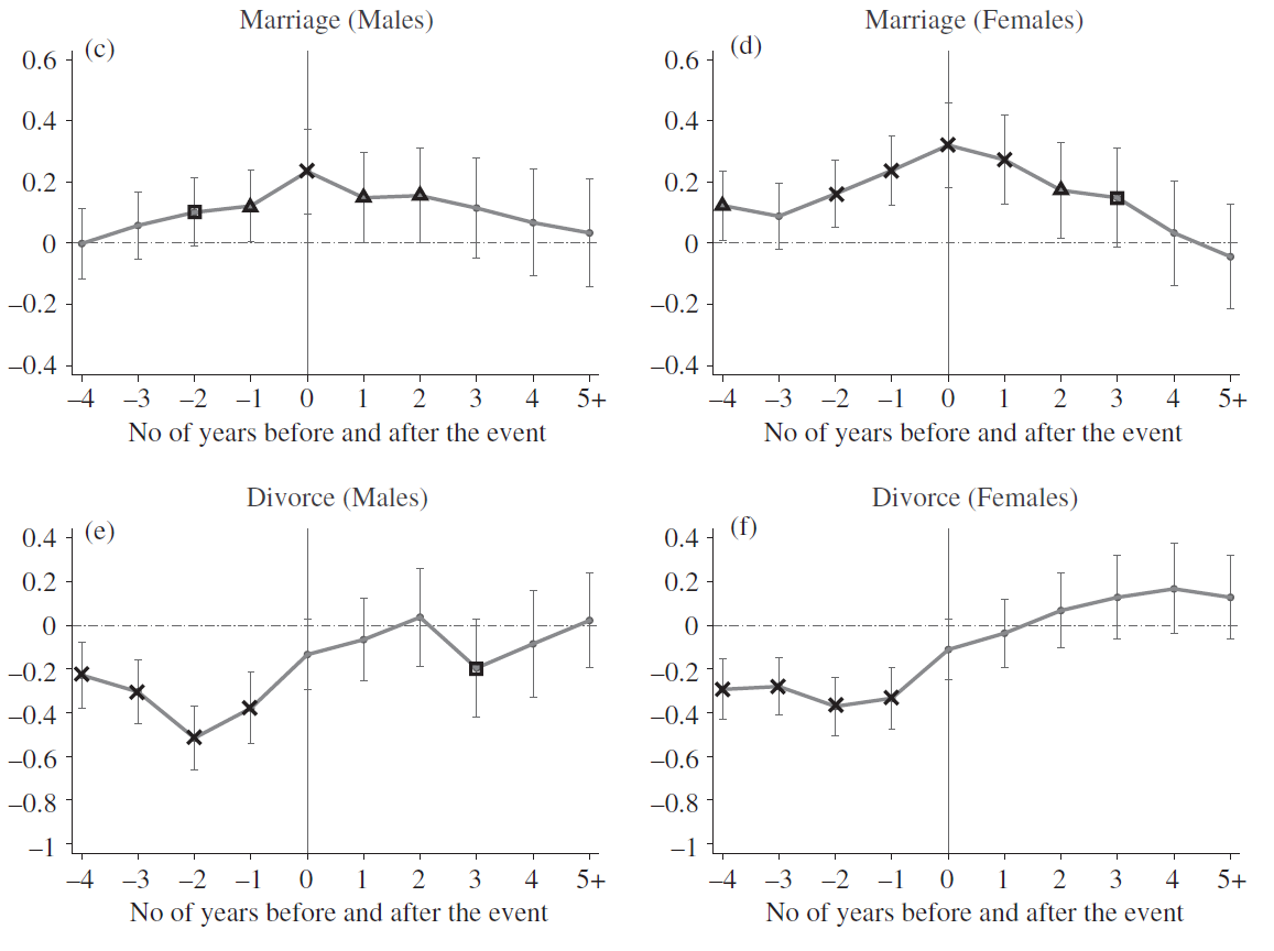
Life course events & Happiness
Clark and Georgellis (2013)
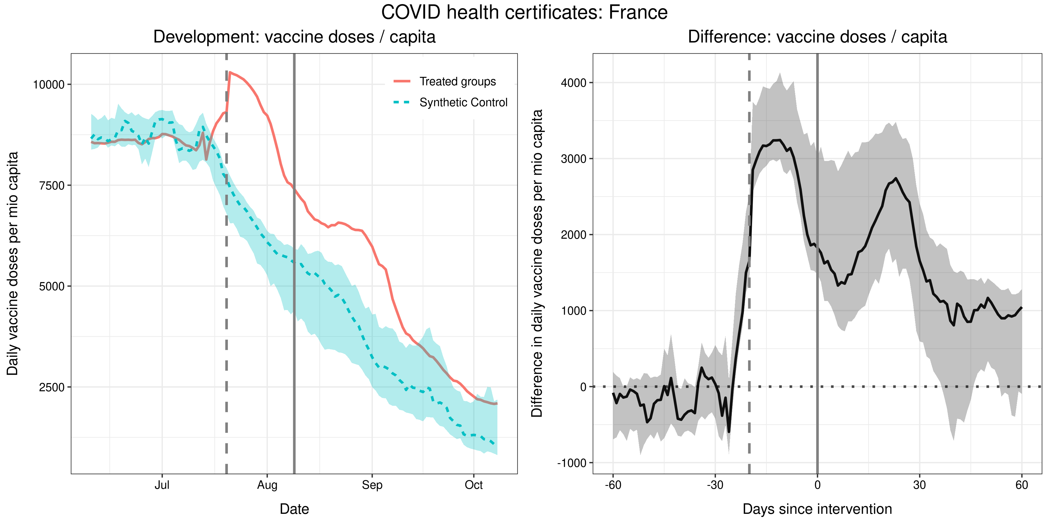
Synthetic Control
Mills and Rüttenauer (2022)