When Can We Use Two-Way Fixed-Effects
2024-06-07
Reviewer 2 is worried
“For staggered interventions, the basic TWFE estimator has come under considerable scrutiny lately” (Wooldridge 2021)
- Bias in TWFE under heterogeneous treatment effects (Goodman-Bacon 2021)
- Several new dynamic DiD estimators
Aims
- (When) Can we still use TWFE?
- How do the new estimators perform under violation of assumptions?
The setup
The 2 \(\times\) 2 Diff-in-Diff with staggered adoption of treatment \(D\):
\[ y_{it} = \alpha + \gamma D_{i} + \lambda Post_{t} + \delta_{DD} (D_{i} \times Post_{t}) + \upsilon_{it}, \]
and the intuitive treatment effect (the difference in differences):
\[ \hat{\delta}_{DD} = \mathrm{E}(\Delta y_{T}) - \mathrm{E}(\Delta y_{C}) = [\mathrm{E}(y_{T}^{post}) - \mathrm{E}(y_{T}^{pre})] - [\mathrm{E}(y_{C}^{post}) - \mathrm{E}(y_{C}^{pre})]. \]
With multiple periods, we would rely on the two-way FE:
\[ y_{it} = \beta_{TWFE} D_{it} + \alpha_i + \zeta_t + \epsilon_{it}. \]
However, what does this two-way FE with multiple periods actually compare?
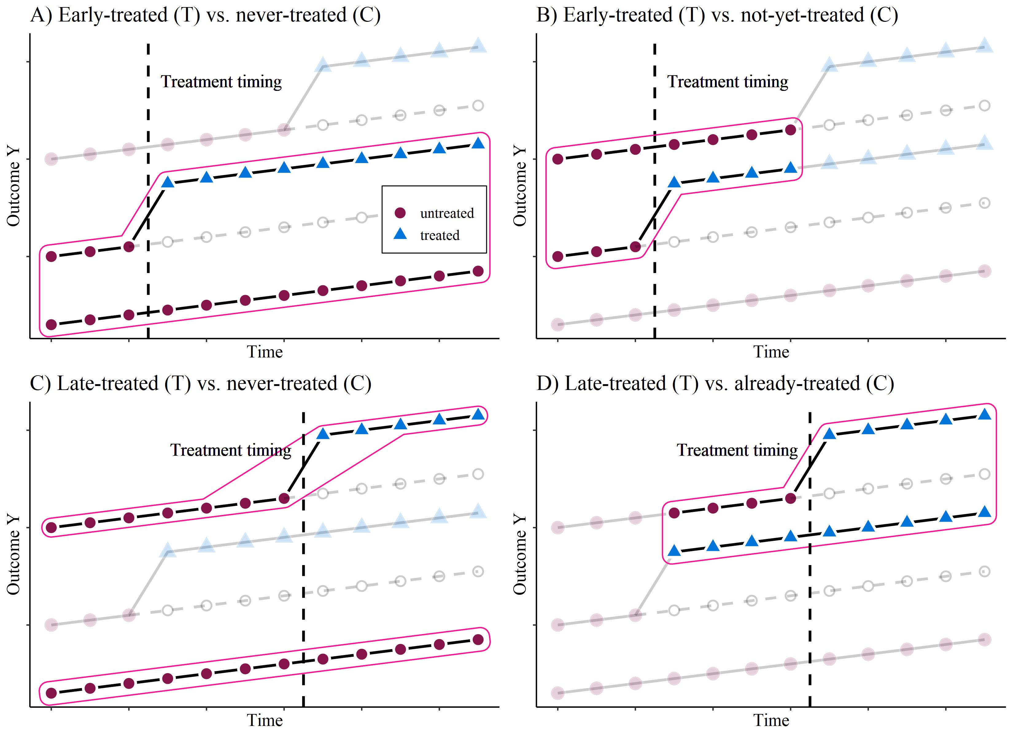
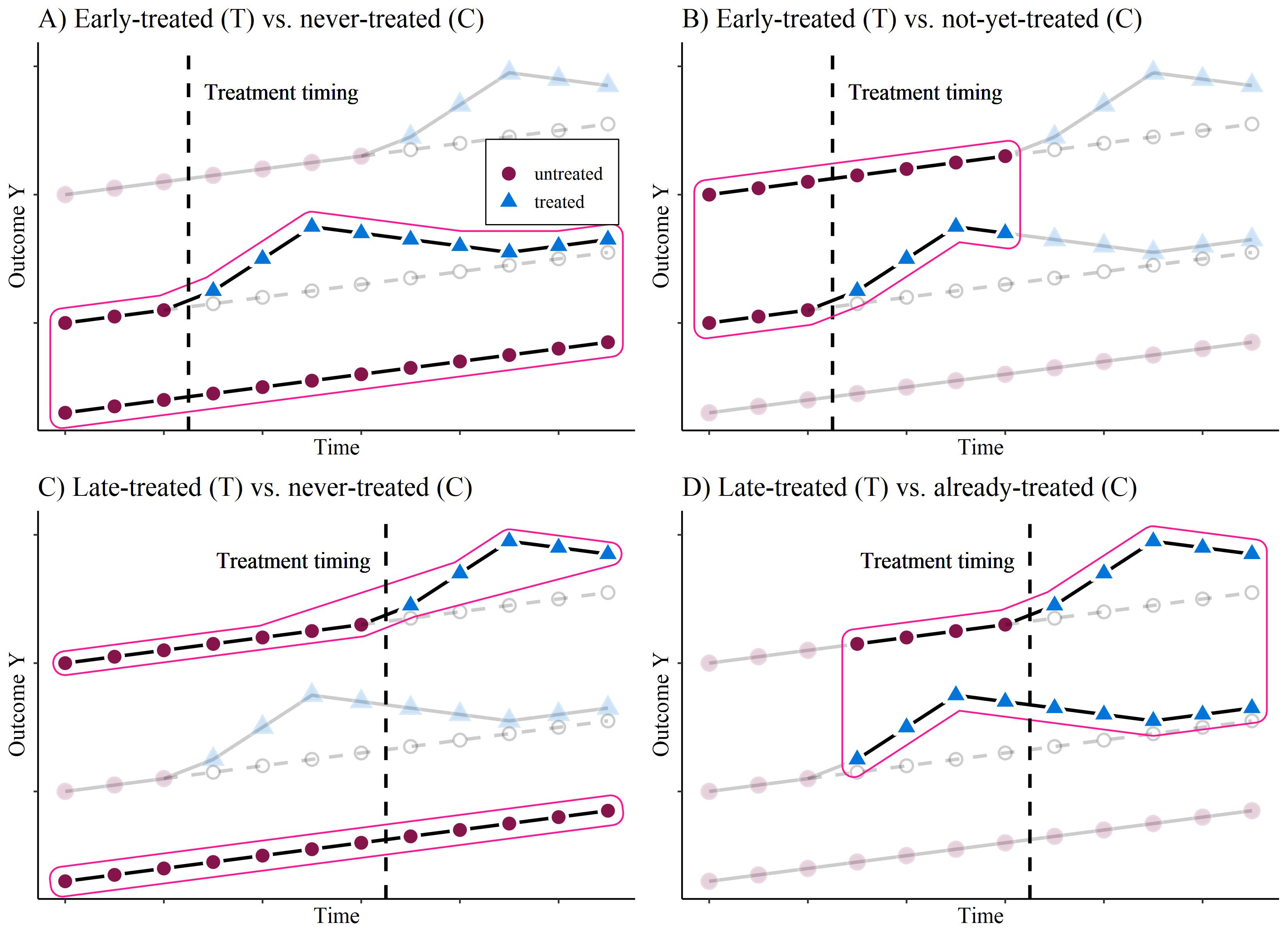
The problem
with 3 groups: 1) Early treated, 2) Late treated, 3) Never treated.

Panel D) is the “forbidden” comparison, see Goodman-Bacon (2021), de Chaisemartin and D’Haultfœuille (2020)
A potential solution
Dynamic Diff-in-Diff (Callaway and Sant’Anna 2020)
- Estimate all single \(2 \times 2\) Diff-in-Diff comparisons
- for each treatment-group \(g\) and time period \(t\)
\[ \delta_{g,t} = \mathrm{E}(\Delta y_{g}) - \mathrm{E}(\Delta y_{C}) = [\mathrm{E}(y_{g}^{t}) - \mathrm{E}(y_{g}^{g-1})] - [\mathrm{E}(y_{C}^{t}) - \mathrm{E}(y_{C}^{g-1})], \]
- where the control group can either be the never-treated or the not-yet-treated.
- Average the ‘good’ comparisons into a single / time-specific treatment measure
\[ \theta_D(e) := \sum_{g=1}^G \mathbf{1} \{ g + e \leq T \} \delta(g,g+e) P(G=g | G+e \leq T), \]
- where \(e\) specifies for how long a unit has been exposed to the treatment.
A potential solution

Disaggregation based estimators, such as Goodman-Bacon (2021)
The Monte Carlo Simulations
The Monte Carlo setup
- N = 500, T = 15, R = 1,000
- Estimators:
- TWFE
- Matrix Completion (Athey et al. 2021)
- Callaway & SantAnna (Callaway and Sant’Anna 2020)
- Sun & Abraham (Sun and Abraham 2021)
- Borusiak (Borusyak, Jaravel, and Spiess 2021)
- Wooldridge ETWFE (Wooldridge 2021)
| Set-up | effect over time | effect structure | anticipation | trended omv | parallel trends |
|---|---|---|---|---|---|
| 1 | homogeneous | step-level shift | no | no | yes |
| 2 | heterogeneous | trend breaking | no | no | yes |
| 3 | heterogeneous | inverted-U shaped | no | no | yes |
| 4 | heterogeneous | inverted-U shaped | negative | no | yes |
| 5 | heterogeneous | inverted-U shaped | no | yes | yes |
| 6 | heterogeneous | inverted-U shaped | no | no | no |
Single Treatment Measure

Single Treatment Measure

Event-time design
- Inverted U-shape

Event-time design
- Anticipation

Event-time design
- Non-parallel trends

Conclusions
The bias in TWFE
- is mainly a problem of specification, not the estimator itself
- can be overcome by using an event study specification
There are others problems that are harder to address:
- Parallel Trends
- No Anticipation
Differences between novel Diff-in-Diff estimators
- Callaway SantAnna / Sun Abraham more sensitive to anticipation
- Borusyak / Wooldridge / Matrix Completion more sensitive to parallel trends
Conclusions

References
More results
Event-time design
- Homogeneous treatment effect

Event-time design
- Trend breaking

Event-time design
- Trending OMV

Fixed Effects Individuals Slopes
- Inverted U-shape & 6. Non-parallel trends

More theory
Homogeneous treatment effect
Multiple Treatment TWFE according to Goodman-Bacon (2021)
Trend-breaking treatment effect
Multiple Treatment TWFE according to Goodman-Bacon (2021)
Inverse u-shaped treatment effect
Multiple Treatment TWFE according to Goodman-Bacon (2021)
Forbidden comparison

‘Forbidden’ comparison in homogeneous vs heterogeneous treatment effect
Disaggregation based estimators
The Sun and Abraham (2021) estimator calculates the cohort-specific average treatment effect on the treated \(CATT_{e,\ell}\) for \(\ell\) periods from the initial treatment and for the cohort of units first treated at time \(e\). These cohort-specific and time-specific estimates are the average based on their sample weights.
The algorithm
- Estimate \(CATT_{e,\ell}\) with a two-way fixed effects estimator that interacts the cohort and relative period indicators
\[ Y_{i,t} =\alpha_{i}+\lambda_{t}+\sum_{e\not\in C}\sum_{\ell\neq-1}\delta_{e,\ell}(\mathbf{1}\{E_{i}=e\}\cdot D_{i,t}^{\ell})+\epsilon_{i,t}. \]
The control group cohort \(C\) can either be the never-treated, or (if they don’t exist), Sun and Abraham (2021) propose to use the latest-treated cohort as control group. By default, the reference period is the relative period before the treatment \(\ell=-1\).
Calculate the sample weights of the cohort within each relative time period \(Pr\{E_{i}=e\mid E_{i}\in[-\ell,T-\ell]\}\)
Use the estimated coefficients from step 1) \(\widehat{\delta}_{e,\ell}\) and the estimated weights from step 2) \(\widehat{Pr}\{E_{i}=e\mid E_{i}\in[-\ell,T-\ell]\}\) to calculate the interaction-weighted estimator \(\widehat{\nu}_{g}\):
\[ \widehat{\nu}_{g}=\frac{1}{\left|g\right|}\sum_{\ell\in g}\sum_{e}\widehat{\delta}_{e,\ell}\widehat{Pr}\{E_{i}=e\mid E_{i}\in[-\ell,T-\ell]\} \]
This is similar to a ‘parametric’ (although very flexible) version of Callaway and Sant’Anna (2020).
Imputation based methods
This comes from Golub Capital Social Impact Lab ML Tutorial
Horizontal Regression and Unconfoundedness literature
The unconfoundedness literature focuses on the single-treated-period structure with a thin matrix (\(N \gg T\)), a substantial number of treated and control units, and imputes the missing potential outcomes using control units with similar lagged outcomes. So \(Y_{iT}\) is missing for some \(i\) (\(N_t\) “treated units”) and no missing entries for other units (\(N_c = N - N_t\) “control units”):
\[ Y_{N\times T}=\left( \begin{array}{ccccccc} \checkmark & \checkmark & \checkmark \\ \checkmark & \checkmark & \checkmark \\ \checkmark & \checkmark & {\color{red} ?} \\ \checkmark & \checkmark & {\color{red} ?} \\ \checkmark & \checkmark & \checkmark \\ \vdots & \vdots &\vdots \\ \checkmark & \checkmark & {\color{red} ?} \\ \end{array} \right)\hskip1cm W_{N\times T}=\left( \begin{array}{ccccccc} 1 & 1 & 1 \\ 1 & 1 & 1 \\ 1 & 1 & 0 \\ 1 & 1 & 0 \\ 1 & 1 & 1 \\ \vdots & \vdots &\vdots \\ 1 & 1 & 0 \\ \end{array} \right) \]
For treated units, the predicted outcome is:
\[ \hat Y_{iT}=\hat \beta_0+\sum_{s=1}^{T-1} \hat \beta_s Y_{Nt}, \]
where
\[ \hat\beta= \arg\min_{\beta} \sum_{i:(i,T)\in \cal{O}}(Y_{iT}-\beta_0-\sum_{s=1}^{T-1}\beta_s Y_{is})^2. \]
A simple version of the unconfoundedness approach is to regress the last period outcome on the lagged outcomes. A more advances version would be matching.
Vertical Regression and the Synthetic Control literature
The synthetic control methods focus primarily on the single-treated-unit block structure with a relatively fat (\(T\gg N\)) or approximately square (\(T\approx N\)) matrix. \(Y_{Nt}\) is missing for \(t \geq T_0\) and there are no missing entries for other units:
\[ Y_{N\times T}=\left( \begin{array}{ccccccc} \checkmark & \checkmark & \checkmark & \dots & \checkmark \\ \checkmark & \checkmark & \checkmark & \dots & \checkmark \\ \checkmark & \checkmark & {\color{red} ?} & \dots & {\color{red} ?} \\ \end{array} \right)\hskip0.5cm W_{N\times T}=\left( \begin{array}{ccccccc} 1 & 1 & 1 & \dots & 1 \\ 1 & 1 & 1 & \dots & 1 \\ 1 & 1 & 0 & \dots & 0 \\ \end{array} \right) \]
For the treated unit in period \(t\), for \(t=T_0, ..., T\), the predicted outcome is:
\[ \hat Y_{Nt}=\hat \omega_0+\sum_{i=1}^{N-1} \hat \omega_i Y_{it} \]
where
\[ \hat\omega= \arg\min_{\omega} \sum_{t:(N,t)\in \cal{O}}(Y_{Nt}-\omega_0-\sum_{i=1}^{N-1}\omega_i Y_{is})^2. \]
See Athey et al. (2021)
Interactive Factor Models
Generalized Fixed Effects (Interactive Fixed Effects, Factor Models):
\[ Y_{it} = \sum_{r=1}^R \gamma_{ir} \delta_{tr} + \epsilon_{it} \quad \text{or} \quad, \mathbf{Y} = \mathbf U \mathbf V^\mathrm T + \mathbf{\varepsilon}. \]
- with with \(\mathbf U\) being an \(N \times r\) matrix of unknown factor loadings (unit-specific intercepts),
- and \(\mathbf V\) an \(T \times r\) matrix of unobserved common factors (time-varying coefficients).
Estimate \(\\delta\) and \(\\gamma\) by least squares and use to impute missing values.
\[ \hat Y _{NT} = \sum_{r=1}^R \hat \delta_{Nr} \hat \gamma_{rT}. \]
In a matrix form, the \(Y_{N \times T}\) can be rewritten as:
\[ Y_{N\times T}= \mathbf U \mathbf V^\mathrm T + \epsilon_{N \times T} = \mathbf L_{N \times T} + \epsilon_{N \times T} = \\ \left( \begin{array}{ccccccc} \delta_{11} & \dots & \delta_{R1} \\ \vdots & \dots & \vdots \\ \vdots & \dots & \vdots \\ \vdots & \dots & \vdots \\ \delta_{1N} & \dots & \delta_{RN} \\ \end{array}\right) \left( \begin{array}{ccccccc} \gamma_{11} & \dots \dots \dots & \gamma_{1T} \\ \vdots & \dots \dots \dots & \vdots \\ \gamma_{R1} & \dots \dots \dots & \gamma_{RT} \\ \end{array} \right) + \epsilon_{N \times T} \]
Matrix Completion
Instead of estimating the factors, we estimate the matrix \(\mathbf L_{N \times T}\) directly. It is supposed to generalise the horizontal and vertical approach.
\[ Y_{N\times T}=\left( \begin{array}{cccccccccc} {\color{red} ?} & {\color{red} ?} & {\color{red} ?} & {\color{red} ?} & {\color{red} ?}& \checkmark & \dots & {\color{red} ?}\\ \checkmark & {\color{red} ?} & {\color{red} ?} & {\color{red} ?} & \checkmark & {\color{red} ?} & \dots & \checkmark \\ {\color{red} ?} & \checkmark & {\color{red} ?} & {\color{red} ?} & {\color{red} ?} & {\color{red} ?} & \dots & {\color{red} ?} \\ {\color{red} ?} & {\color{red} ?} & {\color{red} ?} & {\color{red} ?} & {\color{red} ?}& \checkmark & \dots & {\color{red} ?}\\ \checkmark & {\color{red} ?} & {\color{red} ?} & {\color{red} ?} & {\color{red} ?} & {\color{red} ?} & \dots & \checkmark \\ {\color{red} ?} & \checkmark & {\color{red} ?} & {\color{red} ?} & {\color{red} ?} & {\color{red} ?} & \dots & {\color{red} ?} \\ \vdots & \vdots & \vdots &\vdots & \vdots & \vdots &\ddots &\vdots \\ {\color{red} ?} & {\color{red} ?} & {\color{red} ?} & {\color{red} ?}& \checkmark & {\color{red} ?} & \dots & {\color{red} ?}\\ \end{array} \right) \]
This can be done via Nuclear Norm Minimization:
\[ \min_{L}\frac{1}{|\cal{O}|} \sum_{(i,t) \in \cal{o}} \left(Y_{it} - L_{it} \right)^2+\lambda_L \|L\|_* \]
- where \(\cal{O}\) denote the set of pairs of indices corresponding to the observed entries (the entries with \(W_{it} = 0\)).
Given any \(N\times T\) matrix \(A\), define the two \(N\times T\) matrices \(P_\cal{O}(A)\) and \(P_\cal{O}^\perp(A)\) with typical elements: \[ P_\cal{O}(A)_{it}= \left\{ \begin{array}{ll} A_{it}\hskip1cm & {\rm if}\ (i,t)\in\cal{O}\,,\\ 0&{\rm if}\ (i,t)\notin\cal{O}\,, \end{array}\right. \] and \[ P_\cal{O}^\perp(A)_{it}= \left\{ \begin{array}{ll} 0\hskip1cm & {\rm if}\ (i,t)\in\cal{O}\,,\\ A_{it}&{\rm if}\ (i,t)\notin\cal{O}\,. \end{array}\right. \]
Let \(A=S\Sigma R^\top\) be the Singular Value Decomposition for \(A\), with \(\sigma_1(A),\ldots,\sigma_{\min(N,T)}(A)\), denoting the singular values. Then define the matrix shrinkage operator \[ \ shrink_\lambda(A)=S \tilde\Sigma R^\top\,, \] where \(\tilde\Sigma\) is equal to \(\Sigma\) with the \(i\)-th singular value \(\sigma_i(A)\) replaced by \(\max(\sigma_i(A)-\lambda,0)\).
The algorithm
- Start with the initial choice \(L_1(\lambda)=P_\cal{O}(Y)\), with zeros for the missing values.
- Then for \(k=1,2,\ldots,\) define, \[ L_{k+1}(\lambda)=shrink_\lambda\Biggl\{P_\cal{O}(Y)+P_\cal{O}^\perp\Big(L_k(\lambda)\Big)\Biggr\}\, \] until the sequence \(\left\{L_k(\lambda)\right\}_{k\ge 1}\) converges.
- The limiting matrix \(L^*\) is our estimator for the regularization parameter \(\lambda\), denoted by \(\hat{L}(\lambda,\cal{O})\).
Borusyak DiD imputation
We start with the assumption that we can write the underlying model as:
\[ Y_{it} = A_{it}^{'}\lambda_i + X_{it}^{'}\delta + D_{it}^{'}\Gamma_{it}^{'}\theta + \varepsilon_{it} \]
- where \(A_{it}^{'}\lambda_i\) contains unit FEs, but also allows to interact them with some observed covariates unaffected by the treatment status
- and \(X_{it}^{'}\delta\) nests period FEs but additionally allows any time-varying covariates,
- \(\lambda_i\) is a vector of unit-specific nuisance parameters,
- and \(\delta\) is a vector of nuisance parameters associated with common covariates.
The algorithm
- For every treated observation, estimate expected untreated potential outcomes \(A_{it}^{'}\lambda_i + X_{it}^{'}\delta\) by some unbiased linear estimator \(\hat Y_{it}(0)\) using data from the untreated observations only,
- For each treated observation (\(\in\Omega_1\)), set \(\hat\tau_{it} = Y_{it} - \hat{Y}_{it}(0)\),
- Estimate the target by a weighted sum \(\hat\tau = \sum_{it\in\Omega_1}w_{it}\hat\tau_{it}\).
See Borusyak, Jaravel, and Spiess (2021).
Note that this uses all pre-treatment periods (also those further away) for imputation of the counterfactual.
Fixed Effects Individual Slopes (FEIS)
FEIS allows to control for heterogeneous slopes in addition to time-constant heterogeneity (Rüttenauer and Ludwig 2023)
\[ y_{it} =\boldsymbol{\mathbf{X}}_{it}\beta + \boldsymbol{\mathbf{W}}_{it}\alpha_i + \epsilon_{it}, \]
- where \(W_{it}\) consists of a constant term and \(k\) additional slope variables, and
- \(\alpha_i\) is a \(k+1\) vector of individual-specific coefficients for the unit FE and \(k\) slope variables.
The algorithm
- estimate the individual-specific predicted values for the dependent variable and each covariate based on an individual intercept and the additional slope variables of \(\boldsymbol{\mathbf{W}}_i\),
- ‘detrend’ the original data by these individual-specific predicted values \[ y_{it} - \hat{y}_{it}, \\ \boldsymbol{\mathbf{x}}_{it} - \hat{\boldsymbol{\mathbf{x}}}_{it}, \]
- and run an OLS model on the residual (‘detrended’) data.
For computational reasons, this is done using the the ‘residual maker’ matrix \(\boldsymbol{\mathbf{M}}_i = \boldsymbol{\mathbf{I}}_T - \boldsymbol{\mathbf{W}}_i(\boldsymbol{\mathbf{W}}^\intercal_i \boldsymbol{\mathbf{W}}_i)^{-1}\boldsymbol{\mathbf{W}}^\intercal_i\): \[ \begin{align} y_{it} - \hat{y}_{it} =& (\boldsymbol{\mathbf{x}}_{it} - \hat{\boldsymbol{\mathbf{x}}}_{it})\boldsymbol{\mathbf{\beta }}+ \epsilon_{it} - \hat{\epsilon}_{it}, \\ \boldsymbol{\mathbf{M}}_i \boldsymbol{\mathbf{y}}_i =& \boldsymbol{\mathbf{M}}_i \boldsymbol{\mathbf{X}}_i\boldsymbol{\mathbf{\beta }}+ \boldsymbol{\mathbf{M}}_i \boldsymbol{\mathbf{\epsilon}}_{i}, \\ \tilde{\boldsymbol{\mathbf{y}}}_{i} =& \tilde{\boldsymbol{\mathbf{X}}}_{i}\boldsymbol{\mathbf{\beta }}+ \tilde{\boldsymbol{\mathbf{\epsilon}}}_{i}, \end{align} \]