Panel Data Estimators 1

Tobias Rüttenauer

Variance Decomposition

Age and happiness

Let’s clarify the idea and advantage of panel data with an example.

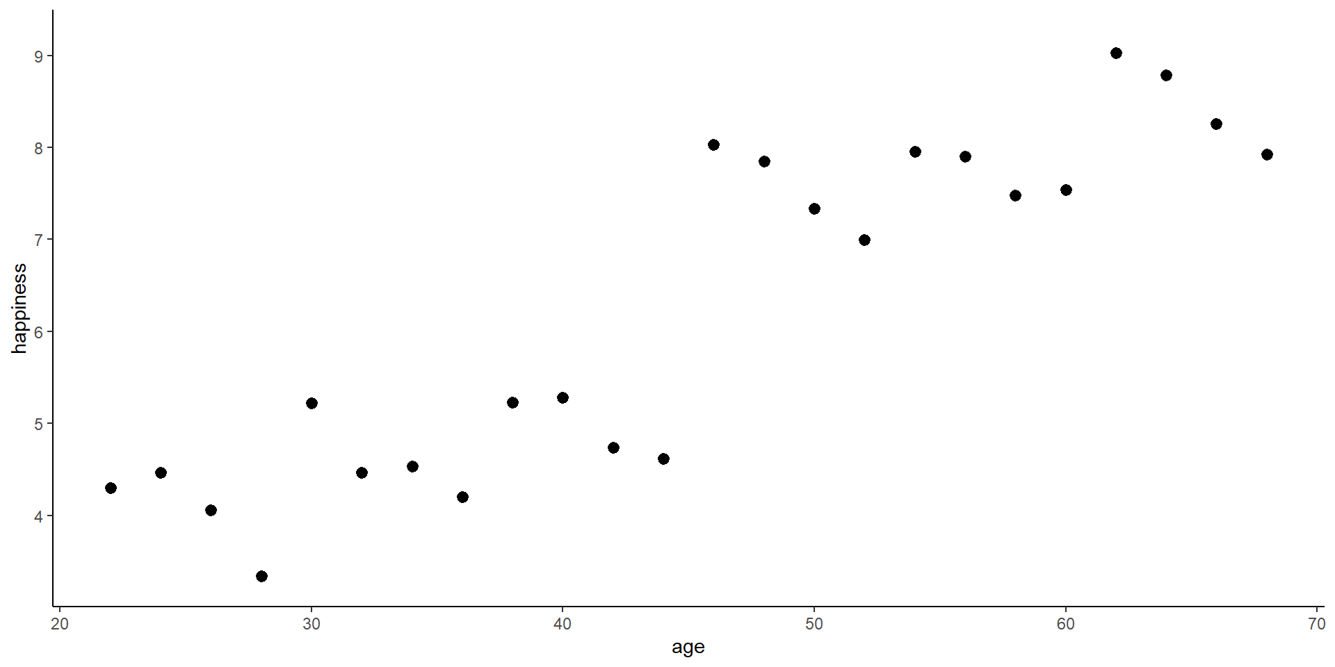
Assume we want to know the relationship between age (as our independent variable) and happiness (as our dependent variable), and we have data on 24 observations.

Code

################################
### Example 1: Age happiness ###
################################

set.seed(213)

### Data simulation program
simdata <- function(N = 6, T = 4,
                    age_range = c(20:60), 
                    u_sd = 0.2, uw_sd = 0){
  
  # id and wave
  df <- data.frame(matrix(NA, ncol = 2, nrow = N*T))
  names(df) <- c("id", "time")
  
  df$id <- rep(1:N, each = T)
  df$time <- rep(1:T, times = N)
  df$idname <- factor(df$id, levels = c(1:N), labels = paste("Person", c(1:N)))
  
  # age
  startingage <- age_range
  startingage <- round(quantile(startingage, probs = seq(0, 1, 1/(N-1))), 0)
  df$age <- unname(rep(startingage, each = T)) + df$time*2
  
  # cohort 
  df$cohort <- 0
  df$cohort[(N*T/2 + 1):(N*T)] <- 1
  df$cohort <- factor(df$cohort, levels = c(0, 1), 
                      labels = c("Younger cohort", "Older cohort"))
  
  # demeaned age
  df$dm_age <- df$age - ave(df$age, df$id, FUN = function(x) mean(x)) 
  
  # Personal intercept
  df$intercept <- 5 + 0.5 * df$id
  
  # Overall error
  u <- rnorm(N*T, mean = 0, sd = u_sd)
  
  # Additional within error
  uw <- unlist(lapply(1:N, function(x) rnorm(T, mean = 0, sd = uw_sd)))
  
  # Gen happiness
  y <- 1 + 0.05 * df$age - 0.2 * df$dm_age + 2 * as.numeric(df$cohort) + u + uw
  df$happiness <- y
  
  # Gen person means
  df$m_age <- ave(df$age, df$id, FUN = function(x) mean(x)) 
  df$m_happiness <- ave(df$happiness, df$id, FUN = function(x) mean(x)) 
  
  return(df)
}

### Set up six individuals with age and happiness
N <- 6
T <- 4

df <- simdata(N = N, T = T)


# Total line for plot
lm1 <- lm(happiness ~ age, data = df)
lm2 <- lm(happiness ~ age + cohort, data = df)
lm3 <- lm(happiness ~ age + idname, data = df)
lm4 <- lm(m_happiness ~ m_age, data = df)

Age and happiness

Code

zp0 <- ggplot(df, aes(age, happiness)) +
  geom_point( aes(x = age, y = happiness), size = 2, stroke = 1) +
  ylim(3.3, 9.2) + expand_limits(y = c(0, 0)) + 
  theme_classic() +
  theme(legend.key = element_blank(), legend.title = element_blank(),
        legend.position = c(0.95,0.05), legend.justification = c("right", "bottom"),
        legend.background = element_blank(),
        legend.box.background = element_rect(colour = "black"))
zp0  

Cross-sectional setting

In a cross-sectional setting, we could just run a standard linear regression model using Omitted Least Squares (OLS) of the form

\[ y_{i} = \alpha + \beta_1 x_{i} + \upsilon_{i}, \]

where \(y_{i}\) is the dependent variable (happiness) and \(x_i\) the independent variable of each observation \(i \in \{1, \dots, 24\}\). \(\beta_1\) is the coefficient of interest, \(\alpha\) the overall intercept and \(\upsilon_{i}\) the error term.

Cross-sectional setting

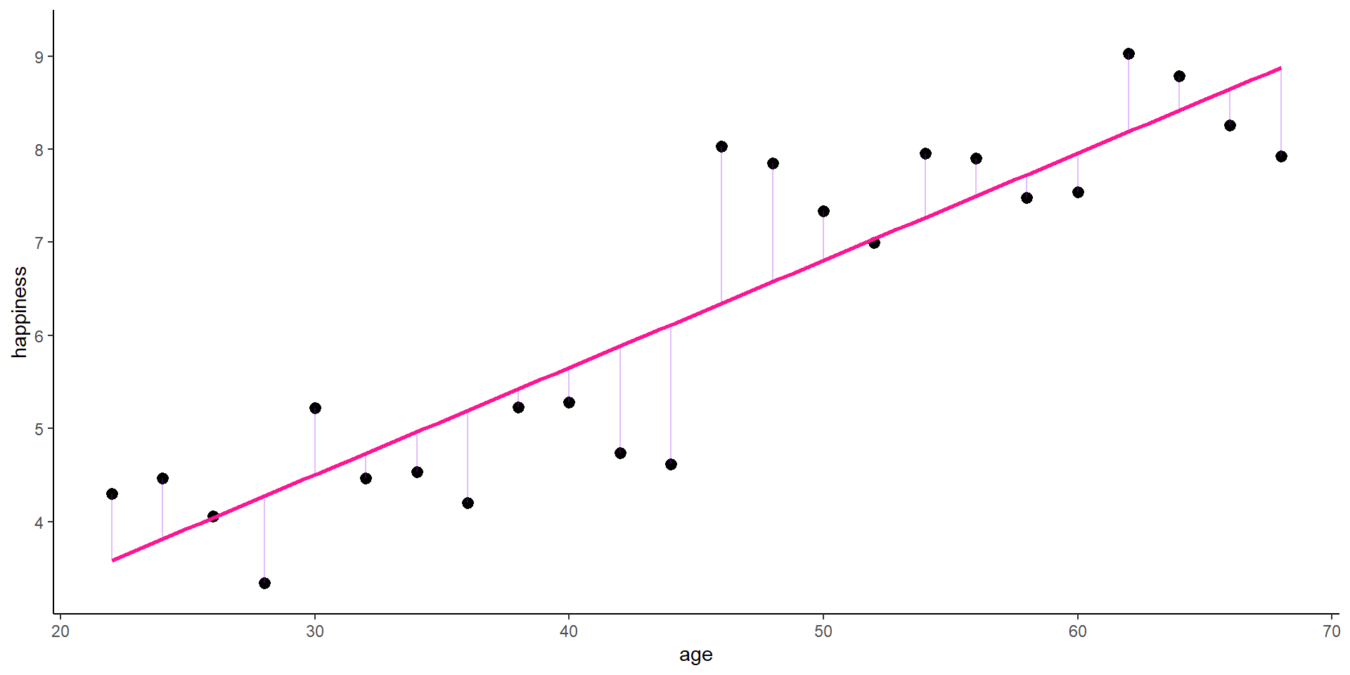
lm1 <- lm(happiness ~ age, data = df)
summary(lm1)

Call:
lm(formula = happiness ~ age, data = df)

Residuals:
    Min      1Q  Median      3Q     Max 
-1.4964 -0.4209 -0.1201  0.6615  1.6868 

Coefficients:
            Estimate Std. Error t value Pr(>|t|)    
(Intercept)   1.0506     0.5696   1.844   0.0787 .  
age           0.1151     0.0121   9.515 2.96e-09 ***
---
Signif. codes:  0 '***' 0.001 '**' 0.01 '*' 0.05 '.' 0.1 ' ' 1

Residual standard error: 0.8206 on 22 degrees of freedom
Multiple R-squared:  0.8045,    Adjusted R-squared:  0.7956 
F-statistic: 90.53 on 1 and 22 DF,  p-value: 2.96e-09

Cross-sectional setting

Code

# The palette with black:
cbp2 <- c("#000000", 
          "#E69F00", 
          "#56B4E9", 
          "#009E73",
          "#F0E442", 
          "#0072B2", 
          "#D55E00", 
          "#CC79A7")

# Save the residual values
df$predicted <- predict(lm1)
df$residuals <- residuals(lm1)

zp1 <- ggplot(df, aes(age, happiness)) +
  geom_point( aes(x = age, y = happiness), size = 2, stroke = 1) +
  geom_smooth(method = 'lm', formula = y ~ x, se = FALSE, color  = "deeppink") +
  geom_segment(data = df, aes(xend = age, yend = predicted), 
               alpha = .3, color = "purple") +
  ylim(3.3, 9.2) + expand_limits(y = c(0, 0)) + 
  theme_classic() +
  theme(legend.key = element_blank(), legend.title = element_blank(),
        legend.position = c(0.95,0.05), legend.justification = c("right", "bottom"),
        legend.background = element_blank(),
        legend.box.background = element_rect(colour = "black"))
zp1  

Adding controls

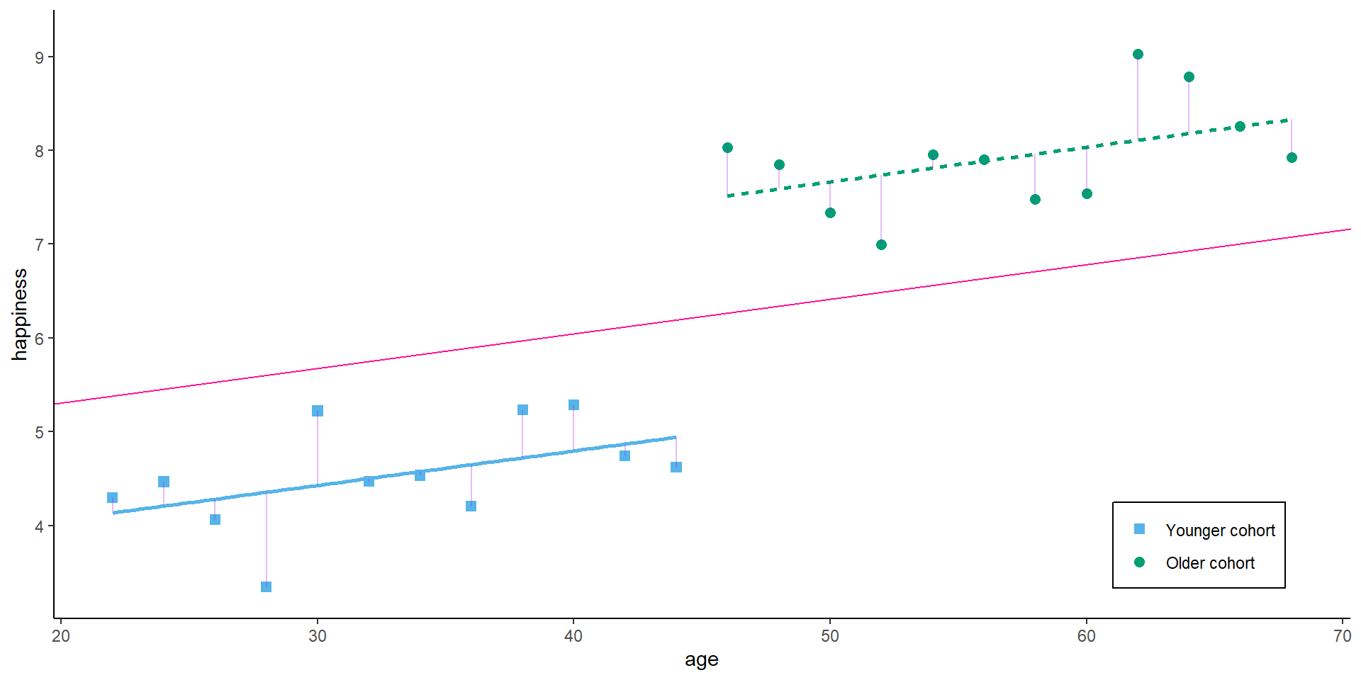
Birth cohort might be a potential confounder that affects age and happiness. We would then estimate the model

\[ y_{i} = \alpha + \beta_1 x_{i} + \beta_2 z_{it} + \upsilon_{i}, \]

where \(z_i\) is the control variable or confounder (cohort).

Adding controls

lm2 <- lm(happiness ~ age + cohort, data = df)
summary(lm2)

Call:
lm(formula = happiness ~ age + cohort, data = df)

Residuals:
     Min       1Q   Median       3Q      Max 
-1.01188 -0.35012 -0.01682  0.31611  0.92289 

Coefficients:
                   Estimate Std. Error t value Pr(>|t|)    
(Intercept)         3.32191    0.52030   6.385 2.50e-06 ***
age                 0.03687    0.01512   2.439   0.0237 *  
cohortOlder cohort  2.49959    0.41862   5.971 6.31e-06 ***
---
Signif. codes:  0 '***' 0.001 '**' 0.01 '*' 0.05 '.' 0.1 ' ' 1

Residual standard error: 0.5114 on 21 degrees of freedom
Multiple R-squared:  0.9275,    Adjusted R-squared:  0.9206 
F-statistic: 134.4 on 2 and 21 DF,  p-value: 1.075e-12

Adding controls

Code

# Save the residual values
for(i in unique(df$cohort)){
  oo <- which(df$cohort == i)
  lmt <- lm(happiness ~ age, data = df[oo, ])
  df$predicted[oo] <- predict(lmt)
  df$residuals[oo] <- residuals(lmt)
}


zp2 <- ggplot(df, aes(age, happiness)) +
  geom_point(aes(x = age, y = happiness, shape = cohort, colour = cohort), 
              size = 2, stroke = 1) +
  geom_smooth(method = 'lm', formula = y ~ x, se = FALSE, show.legend = FALSE,
              mapping = aes(colour = cohort, linetype = cohort)) +  
  geom_segment(data = df, aes(xend = age, yend = predicted), 
               alpha = .3, color = "purple") +
  geom_abline(intercept = lm2$coefficients[1] + 0.5 * lm2$coefficients[3], 
                               slope = lm2$coefficients[2], color  = "deeppink") +  
  ylim(3.3, 9.2) + expand_limits(y = c(0, 0)) + 
  scale_colour_manual(values = cbp2[-c(1, 2)]) + 
  scale_fill_manual(values = cbp2[-c(1, 2)]) + 
  scale_shape_manual(values = c(15:18, 25, 20)) +
  theme_classic() +
  theme(legend.key = element_blank(), legend.title = element_blank(),
        legend.position = c(0.95,0.05), legend.justification = c("right", "bottom"),
        legend.background = element_blank(),
        legend.box.background = element_rect(colour = "black"))
zp2  

Panel data setting

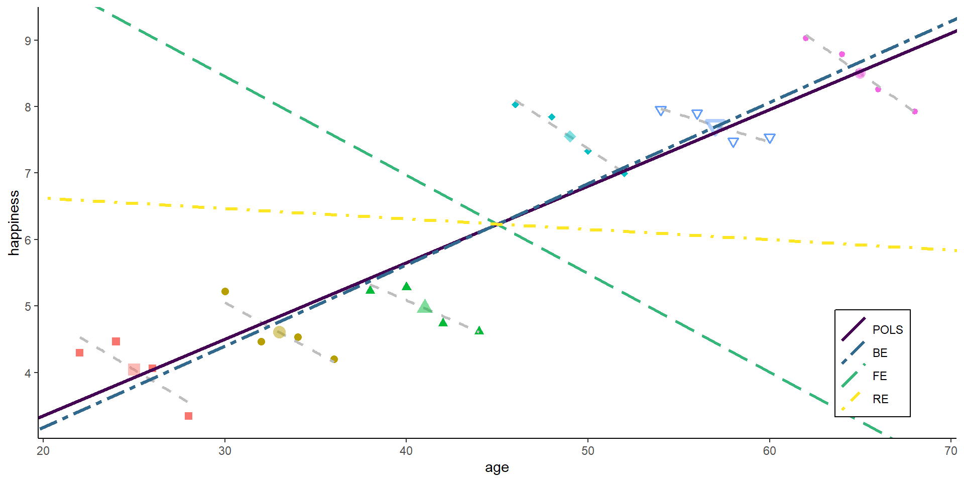
Now, with panel data, we can even go a step further. Assume we would not have observed 24 independent observations, but rather 6 independent individuals (N = 6) at 4 time-points each (T = 4).

Code

zp3 <- ggplot(df, aes(age, happiness)) +
  geom_point( aes(x = age, y = happiness, shape = idname, colour = idname, fill = idname), 
              size = 2, stroke = 1) +
  ylim(3.3, 9.2) + expand_limits(y = c(0, 0)) + 
  scale_colour_manual(values = cbp2[-c(1, 2)]) + 
  scale_fill_manual(values = cbp2[-c(1, 2)]) + 
  scale_shape_manual(values = c(15:18, 25, 20)) +
  theme_classic() +
  theme(legend.key = element_blank(), legend.title = element_blank(),
        legend.position = c(0.95,0.05), legend.justification = c("right", "bottom"),
        legend.background = element_blank(),
        legend.box.background = element_rect(colour = "black"))
zp3 

Panel data setting

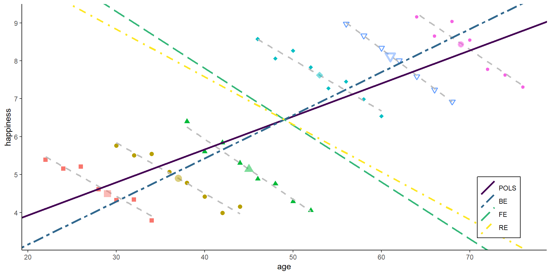
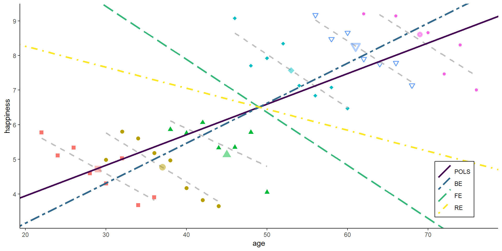
We can then decompose the available variance into three different parts:

• Pooled variance

• Between variance

• Within variance

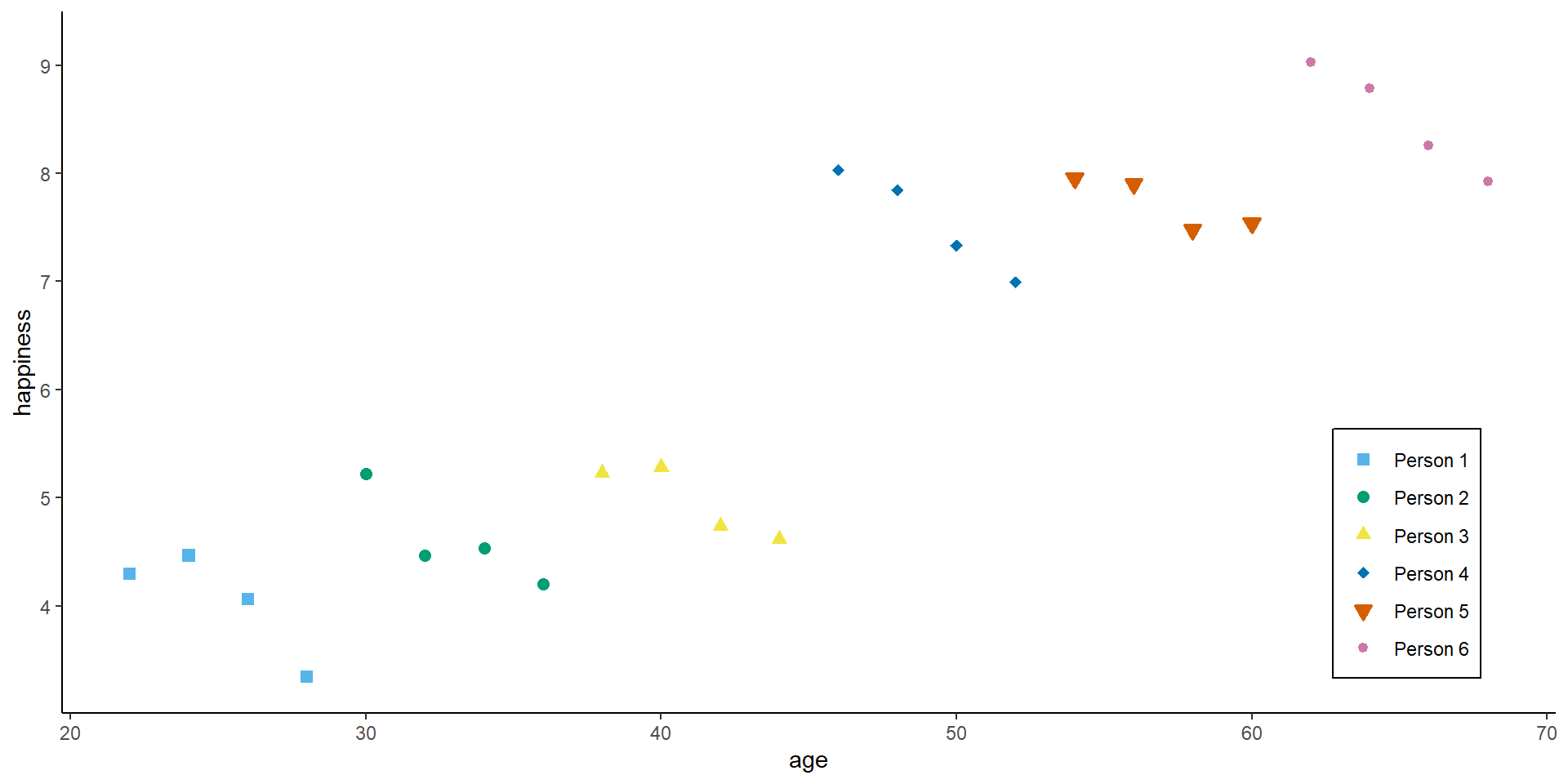
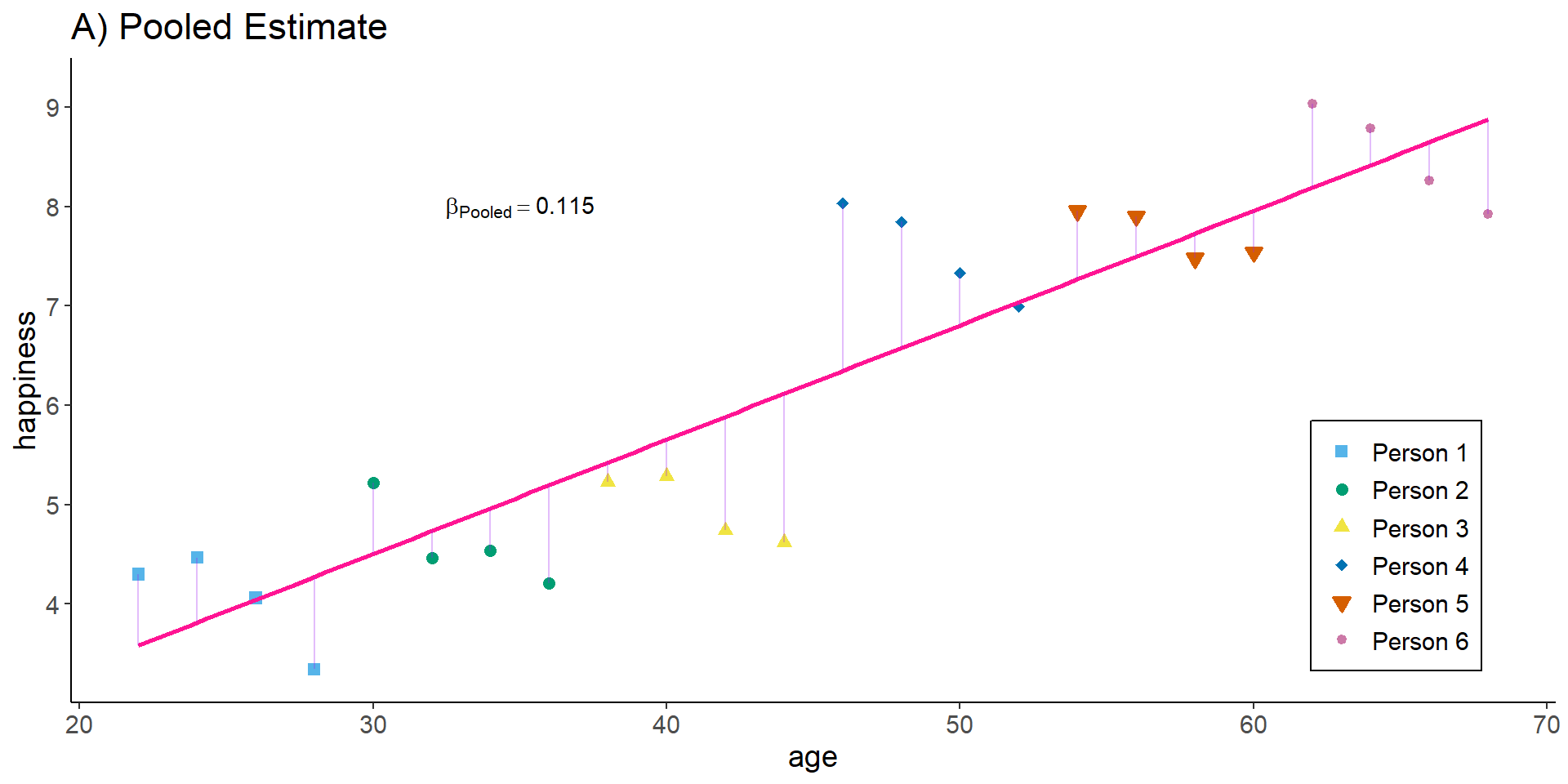
Pooled estimator

The pooled estimator equals what we have seen in the cross-sectional example: we basically assume that we have 24 independent observations and we ignore the person and time dimension. The Pooled OLS estimator is simply:

\[ y_{it} = \alpha + \beta_{POLS} x_{it} + \upsilon_{it}, \]

lm1 <- lm(happiness ~ age, data = df)
summary(lm1)

Pooled estimator

Code

# Save the residual values
df$predicted <- predict(lm1)
df$residuals <- residuals(lm1)

zp3 <- ggplot(df, aes(age, happiness)) +
  geom_point( aes(x = age, y = happiness, shape = idname, colour = idname, fill = idname), 
              size = 2, stroke = 1) +
  geom_smooth(method = 'lm', formula = y ~ x, se = FALSE,
              color  = "deeppink") +
  geom_segment(aes(xend = age, yend = predicted), 
               alpha = .3, color = "purple") +
  annotate("text", x = 35, y = 8.0, 
           label = paste0("beta[Pooled] ==", round(lm1$coefficients[2], 3)), 
           parse = TRUE) +
  ylim(3.3, 9.2) + expand_limits(y = c(0, 0)) + 
  scale_colour_manual(values = cbp2[-c(1, 2)]) + 
  scale_fill_manual(values = cbp2[-c(1, 2)]) + 
  scale_shape_manual(values = c(15:18, 25, 20)) +
  ggtitle("A) Pooled Estimate") +
  theme_classic() +
  theme(legend.key = element_blank(), 
        legend.title = element_blank(),
        text = element_text(size = 14),
        legend.position = c(0.95,0.05), 
        legend.justification = c("right", "bottom"),
        legend.background = element_blank(),
        legend.box.background = element_rect(colour = "black"))
zp3

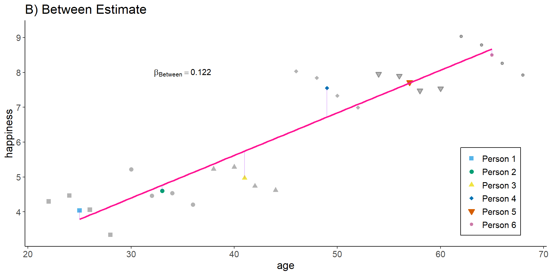
Between estimator

The between estimator only compares different persons and discards the within-person variance. Therefore, we simply run a model that only uses the person-specific means

\[ \bar{y_{i}} = \alpha + \beta_{BTW} \bar{x_{i}} + \bar{\upsilon_{i}}, \]

where \(\bar{y_{i}}\) and \(\bar{x_{i}}\) are the unit-specific means of \(x_{it}\) and \(y_{it}\), respectively.

Between estimator

We can either estimate this by hand:

df$m_happiness <- ave(df$happiness, df$id, FUN = mean)
df$m_age <- ave(df$age, df$id, FUN = mean)

lm2 <- lm(m_happiness ~ m_age, data = df)
summary(lm2)

Between estimator

or we use the plm package to do the job for us

btw2 <- plm(happiness ~ age, data = df,
           index = c("id", "time"),
           effect = "individual", model = "between")
summary(btw2)

Oneway (individual) effect Between Model

Call:
plm(formula = happiness ~ age, data = df, effect = "individual", 
    model = "between", index = c("id", "time"))

Balanced Panel: n = 6, T = 4, N = 24
Observations used in estimation: 6

Residuals:
        1         2         3         4         5         6 
 0.254242 -0.158370 -0.774367  0.831689  0.021989 -0.175184 

Coefficients:
            Estimate Std. Error t-value Pr(>|t|)   
(Intercept) 0.733095   0.834979  0.8780 0.429528   
age         0.122176   0.017755  6.8813 0.002337 **
---
Signif. codes:  0 '***' 0.001 '**' 0.01 '*' 0.05 '.' 0.1 ' ' 1

Total Sum of Squares:    18.13
Residual Sum of Squares: 1.4122
R-Squared:      0.92211
Adj. R-Squared: 0.90263
F-statistic: 47.3519 on 1 and 4 DF, p-value: 0.0023371

Between estimator

Code

df2 <- df
df2$happiness <- df2$m_happiness
df2$age <- df2$m_age
df2 <- df2[which(df2$time == 1), ]

# Save the residual values
lm4 <- lm(m_happiness ~ m_age, data = df2)
df2$predicted <- predict(lm4)
df2$residuals <- residuals(lm4)

zp4 <- ggplot(df, aes(age, happiness)) +
  geom_point(aes(x = age, y = happiness, shape = idname), 
              size = 2, stroke = 1, colour = alpha("black", .3), fill = alpha("black", .3)) +
  geom_point(aes(x = m_age, y = m_happiness, shape = idname, colour = idname,
                 fill = idname), 
             size = 2, stroke = 1) +
  geom_smooth(data = df2, 
              method = 'lm', formula = y ~ x, se = FALSE,
              color  = "deeppink") +
  geom_segment(data = df2, aes(xend = age, yend = predicted), 
               alpha = .3, color = "purple") +
  annotate("text", x = 35, y = 8.0, 
           label = paste0("beta[Between] ==", round(lm4$coefficients[2], 3)), 
           parse = TRUE) +
  ylim(3.3, 9.2) + expand_limits(y = c(0, 0)) + 
  scale_colour_manual(values = cbp2[-c(1, 2)]) + 
  scale_fill_manual(values = cbp2[-c(1, 2)]) + 
  scale_shape_manual(values = c(15:18, 25, 20)) +
  ggtitle("B) Between Estimate") +
  theme_classic() +
  theme(legend.key = element_blank(), 
        legend.title = element_blank(),
        text = element_text(size = 14),
        legend.position = c(0.95,0.05), 
        legend.justification = c("right", "bottom"),
        legend.background = element_blank(),
        legend.box.background = element_rect(colour = "black"))

zp4  

Within estimator

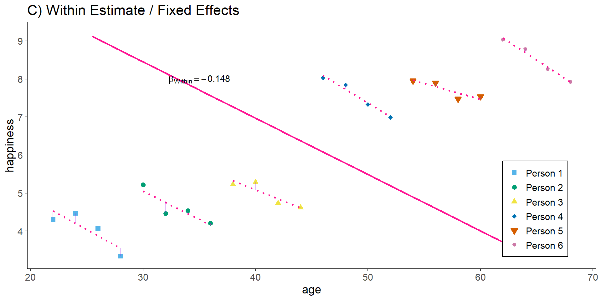
The within estimator only compares different periods within the same person and discards the between-person variance. We could also say the estimator is solely based on changes over time.

\[ y_{it} = \alpha_i + \beta_{WI} x_{it} + \epsilon_{it}, \]

To achieve this, we simply give every person their own intercept \(\alpha_i\): we add a dummy for each person.

Within estimator

Again, we could run this manually

lm3 <- lm(happiness ~ age + idname, data = df)
summary(lm3)

Make sure idname is a factor. Otherwise use as.factor(idname).

Within estimator

or we use plm:

fe1 <- plm(happiness ~ age, data = df,
           index = c("id", "time"),
           effect = "individual", model = "within")
summary(fe1)

• Formula and Data

Within estimator

or we use plm:

fe1 <- plm(happiness ~ age, data = df,
           index = c("id", "time"),
           effect = "individual", model = "within")
summary(fe1)

• Define id and time columns

Within estimator

or we use plm:

fe1 <- plm(happiness ~ age, data = df,
           index = c("id", "time"),
           effect = "individual", model = "within")
summary(fe1)

• effect: Define the type of fixed effects (individual, time, twoways)

• model: Define the estimator (within for FE)

Within estimator

or we use plm:

fe1 <- plm(happiness ~ age, data = df,
           index = c("id", "time"),
           effect = "individual", model = "within")
summary(fe1)

Oneway (individual) effect Within Model

Call:
plm(formula = happiness ~ age, data = df, effect = "individual", 
    model = "within", index = c("id", "time"))

Balanced Panel: n = 6, T = 4, N = 24

Residuals:
     Min.   1st Qu.    Median   3rd Qu.      Max. 
-0.287907 -0.118754  0.035834  0.141721  0.275941 

Coefficients:
     Estimate Std. Error t-value  Pr(>|t|)    
age -0.148245   0.017418 -8.5108 1.556e-07 ***
---
Signif. codes:  0 '***' 0.001 '**' 0.01 '*' 0.05 '.' 0.1 ' ' 1

Total Sum of Squares:    3.2561
Residual Sum of Squares: 0.61893
R-Squared:      0.80992
Adj. R-Squared: 0.74283
F-statistic: 72.4345 on 1 and 17 DF, p-value: 1.5556e-07

Within estimator

Code

df2 <- df
df2$happiness <- df2$happiness - df2$m_happiness + mean(df$happiness)
df2$age <- df2$age - df2$m_age  + mean(df$age)

# Save the residual values
for(i in unique(df$id)){
  oo <- which(df$id == i)
  lmt <- lm(happiness ~ age, data = df[oo, ])
  df$predicted[oo] <- predict(lmt)
  df$residuals[oo] <- residuals(lmt)
}


zp5 <- ggplot(df, aes(age, happiness)) +
  geom_point( aes(x = age, y = happiness, shape = idname, colour = idname, fill  = idname), 
              size = 2, stroke = 1) +
  geom_smooth(method = 'lm', formula = y ~ x, se = FALSE, show.legend = FALSE,
              mapping = aes(group = idname),
              color  = "deeppink", linetype = "dotted") +
  geom_smooth(method = 'lm', formula = y ~ x, se = FALSE, show.legend = FALSE,
              data = df2, color  = "deeppink", fullrange = TRUE) +
  geom_segment(data = df, aes(xend = age, yend = predicted), 
               alpha = .3, color = "purple") +
  annotate("text", x = 35, y = 8.0, 
           label = paste0("beta[Within] ==", round(lm3$coefficients[2], 3)), 
           parse = TRUE) +
  ylim(3.3, 9.2) + expand_limits(y = c(0, 0)) + 
  scale_fill_manual(values = cbp2[-c(1, 2)]) +
  scale_colour_manual(values = cbp2[-c(1, 2)]) + 
  scale_shape_manual(values = c(15:18, 25, 20)) +
  ggtitle("C) Within Estimate / Fixed Effects") +
  theme_classic() +
  theme(legend.key = element_blank(), 
        legend.title = element_blank(),
        text = element_text(size = 14),
        legend.position = c(0.95,0.05), 
        legend.justification = c("right", "bottom"),
        legend.background = element_blank(),
        legend.box.background = element_rect(colour = "black"))

zp5

Comparison

library("texreg")
screenreg(list(lm1, lm2, lm3), digits = 3, 
          custom.model.names = c("POLS", "Between", "Within"))

==================================================
                POLS        Between     Within    
--------------------------------------------------
(Intercept)      1.051       0.733       7.748 ***
                (0.570)     (0.356)     (0.446)   
age              0.115 ***              -0.148 ***
                (0.012)                 (0.017)   
m_age                        0.122 ***            
                            (0.008)               
idnamePerson 2                           1.751 ***
                                        (0.194)   
idnamePerson 3                           3.298 ***
                                        (0.310)   
idnamePerson 4                           7.068 ***
                                        (0.439)   
idnamePerson 5                           8.421 ***
                                        (0.573)   
idnamePerson 6                          10.387 ***
                                        (0.710)   
--------------------------------------------------
R^2              0.805       0.922       0.992    
Adj. R^2         0.796       0.919       0.989    
Num. obs.       24          24          24        
==================================================
*** p < 0.001; ** p < 0.01; * p < 0.05

Comparison

FE: Faster estimation

Often faster than plm: felm() in package lfe

Particularly, with large data, group-specific interactions, or when you want clustered standard error, this can save you time.

FE: Faster estimation

Often faster than plm: felm() in package lfe

library(lfe)
fe1_alt <- felm(happiness ~ age | id | 0 | id,
                data = df)
summary(fe1_alt)

Four-part formula:

• Formula: 1) ordinary covariates, 2) fixed effects, 3) Instrumental Variables, 4) Cluster for SEs

• y ~ x1 + x2 | f1 + f2 | (Q|W ~ x3+x4) | clu1 + clu2

• Can include interactions between FEs: y ~ x1 + x | x:f + f

FE: Faster estimation

Often faster than plm: felm() in package lfe

library(lfe)
fe1_alt <- felm(happiness ~ age | id | 0 | id,
                data = df)
summary(fe1_alt)

Call:
   felm(formula = happiness ~ age | id | 0 | id, data = df) 

Residuals:
     Min       1Q   Median       3Q      Max 
-0.28791 -0.11875  0.03583  0.14172  0.27594 

Coefficients:
    Estimate Cluster s.e. t value Pr(>|t|)    
age -0.14824      0.01711  -8.665 0.000338 ***
---
Signif. codes:  0 '***' 0.001 '**' 0.01 '*' 0.05 '.' 0.1 ' ' 1

Residual standard error: 0.1908 on 17 degrees of freedom
Multiple R-squared(full model): 0.9918   Adjusted R-squared: 0.9889 
Multiple R-squared(proj model): 0.8099   Adjusted R-squared: 0.7428 
F-statistic(full model, *iid*):344.1 on 6 and 17 DF, p-value: < 2.2e-16 
F-statistic(proj model): 75.08 on 1 and 5 DF, p-value: 0.0003384 

Fixed Effects

Assumption for conistency of POLS

The POLS

\[ y_{it} = \alpha + \beta x_{it} + \upsilon_{it} \]

relies on very strong assumptions for consistency, most importantly: The error (including omitted variables) must not be correlated with \(x_{it}\).

• \(\mathrm{E}(\upsilon_{it} | x_{it}) = 0\), or \(Cov(x_{it}, \upsilon_{it}) = 0\)

Marriage and income

Imagine we want to know how getting married affects a persons happiness or their income. POLS (and the between estimator) compare people who eventually get married to people who never get married.

What could potentially go wrong?

One-way fixed effects

To relax the strong assumption, we can decompose the error into two parts (between and within) and split up our main assumption for consistency:

• \(\mathrm{E}(\alpha_{i} | x_{it}) = 0\): No time-constant unobserved heterogeneity

• \(\mathrm{E}(\epsilon_{it} | x_{it}) = 0\): No time-varying unobserved heterogeneity

One-way fixed effects

The FE

\[ y_{it} = \beta x_{it} + \alpha_i + \epsilon_{it} \]

includes unit-specific fixed effects to account for the first type of heterogeneity. The most basic way of including person-specific dummy variable is called Least Square Dummy variable (LSDV) approach.

See e.g. Wooldridge (2010) or Bruderl.2015.

One-way fixed effects

In practice, we usually use a transformation approach, where we first subtract the between variance by using use the person-specific means:

\[ \begin{split} y_{it} - \bar{y_{i}} &= \beta (x_{it}-\bar{x_{i}}) + (\alpha_i - \alpha_i) + (\epsilon_{it}-\bar{\epsilon_{i}})\\ \tilde{y}_{it} &= \beta \tilde{x}_{it} + \tilde{\epsilon}_{it}. \end{split} \]

One-way fixed effects

The main assumption for consistency now is

• \(\mathrm{E}(\epsilon_{it} | x_{it}, \alpha_i) = 0\)

Idiosyncratic time-variation in \(\epsilon_{it}\) (including time trends in \(y\)) must be uncorrelated with variation in \(x_{it}\) across all time periods. However, \(\mathrm{E}(\alpha_{i} | x_{i})\) can be any function of \(x_i\).

• Time-constant unobserved heterogeneity is allowed

• Only time-varying unobserved heterogeneity biases the estimator

Would one-way FE get it right?

Code

##################################
### Example 2: Marriage Income ###
##################################

### Set up six individuals with age and happiness
N <- 4
T <- 6

# id and wave
df2 <- data.frame(matrix(NA, ncol = 2, nrow = N*T))
names(df2) <- c("id", "time")

df2$id <- rep(1:N, each = T)
df2$time <- rep(1:T, times = N)
df2$idname <- factor(df2$id, levels = c(1:N), labels = paste("Person", c(1:N)))

# Marriage dummy
df2$marriage_ever <- 0 
df2$marriage_ever[(N*T/2 + 1):(N*T)] <- 1

df2$marriage <- df2$marriage_ever * ifelse(df2$time >= 4, 1, 0)

# Starting wage
stw <- c(2000, 5000)
stw <- round(quantile(stw, probs = seq(0, 1, 1/(N-1))), 0)

# wage equation
df2$wage <- unname(rep(stw, each = T)) + (df2$time - 1)*50 + 200 * ifelse(df2$time >=4, 1, 0) + df2$marriage * 500

# counterfactual parallel trend
df2$pti <- unname(rep(stw, each = T)) + (df2$time - 1)*50 
df2$pt <- unname(rep(stw, each = T)) + (df2$time - 1)*50 + 200 * ifelse(df2$time >=4, 1, 0) 
df2$pti[df2$marriage_ever == 0 | df2$time < 3] <- NA
df2$pt[df2$marriage_ever == 0 | df2$time < 3] <- NA


### Add individual slope / heterogeneous time trends

# wage equation
df2$wage2 <- unname(rep(stw, each = T)) + (df2$time - 1)*50  + (df2$time - 1)*150*df2$marriage_ever + 200 * ifelse(df2$time >=4, 1, 0) + df2$marriage * 500

# parallel trend
df2$pt2 <- unname(rep(stw, each = T)) + (df2$time - 1)*50 + 200 * ifelse(df2$time >=4, 1, 0) + 2*150
df2$pt2[df2$marriage_ever == 0 | df2$time < 3] <- NA

# actual trend
df2$pt2_cr <- unname(rep(stw, each = T)) + (df2$time - 1)*50 + (df2$time - 1)*150*df2$marriage_ever + 200 * ifelse(df2$time >=4, 1, 0)
df2$pt2_cr[df2$marriage_ever == 0 | df2$time < 3] <- NA

# Marry to factor
df2$marriage <- factor(df2$marriage, levels = c(0, 1), labels = c("not married", "married"))
df2$marriage_ever <- as.factor(df2$marriage_ever)


### Plot 
zp1 <- ggplot(df2, aes(time, wage)) +
  geom_line(aes(x = time, y = wage, group = id), lty = "solid", colour = "black", lwd = 1) + 
  geom_point( aes(x = time, y = wage, shape = marriage, fill = marriage), 
             size = 4, stroke = 1.5, color = "white") +
  theme_classic() +
  scale_shape_manual(values = c(21, 24)) +
  scale_fill_manual(values = c("#85144b", "#0074D9")) +
  scale_color_manual(values = c("#85144b", "#0074D9")) +
  theme(legend.key = element_blank(), legend.title = element_blank(),
        legend.position = c(0.05,0.95), legend.justification = c("left", "top"),
        legend.background = element_blank(),
        legend.box.background = element_rect(colour = "black"),
        legend.spacing.y = unit(-0.1, "cm"))
zp1 

Would one-way FE get it right?

fe2 <- plm(wage ~ marriage, data = df2,
           index = c("id", "time"),
           effect = "individual", model = "within")
summary(fe2)

Oneway (individual) effect Within Model

Call:
plm(formula = wage ~ marriage, data = df2, effect = "individual", 
    model = "within", index = c("id", "time"))

Balanced Panel: n = 4, T = 6, N = 24

Residuals:
   Min. 1st Qu.  Median 3rd Qu.    Max. 
-225.00  -68.75    0.00   68.75  225.00 

Coefficients:
                Estimate Std. Error t-value  Pr(>|t|)    
marriagemarried  850.000     84.552  10.053 4.834e-09 ***
---
Signif. codes:  0 '***' 0.001 '**' 0.01 '*' 0.05 '.' 0.1 ' ' 1

Total Sum of Squares:    2575000
Residual Sum of Squares: 407500
R-Squared:      0.84175
Adj. R-Squared: 0.80843
F-statistic: 101.061 on 1 and 19 DF, p-value: 4.8337e-09

Would one-way FE get it right?

FE is based on within-unit variance.

Note

A one-ways FE would effectively drop all those observations without within-variance on the independent variables. In our case, we would disregard those who never marry.

However, the never married also experienced an increase in wages when the other two married.

Would one-way FE get it right?

Code

### Plot 
zp3 <- ggplot(df2, aes(time, wage)) +
  geom_line(aes(x = time, y = wage, group = id, alpha = marriage_ever), lty = "solid", colour = "black", lwd = 1) + 
  geom_point( aes(x = time, y = wage, shape = marriage, fill = marriage, alpha = marriage_ever), 
              size = 4, stroke = 1.5, color = "white") +
  geom_line(aes(x = time, y = pti, group = id, linetype = "dashed"), colour = "blue", lwd = 1) +
  scale_linetype_identity(labels = "Counterfactual", guide = "legend") +
  scale_alpha_manual(values = c(0.5, 1), guide = "none") +
  # geom_mark_hull(data = df2[df2$marriage_ever == 1, ], aes(x = time, y = wage, fill = marriage),
  #                expand = 0.01, show.legend = FALSE, colour = NA) + 
  theme_classic() +
  scale_shape_manual(values = c(21, 24)) +
  scale_fill_manual(values = c("#85144b", "#0074D9")) +
  scale_color_manual(values = c("#85144b", "#0074D9")) +
  theme(legend.key = element_blank(), legend.title = element_blank(),
        legend.position = c(0.05,0.95), legend.justification = c("left", "top"),
        legend.background = element_blank(),
        legend.box.background = element_rect(colour = "black"),
        legend.spacing.y = unit(-0.1, "cm"))
zp3

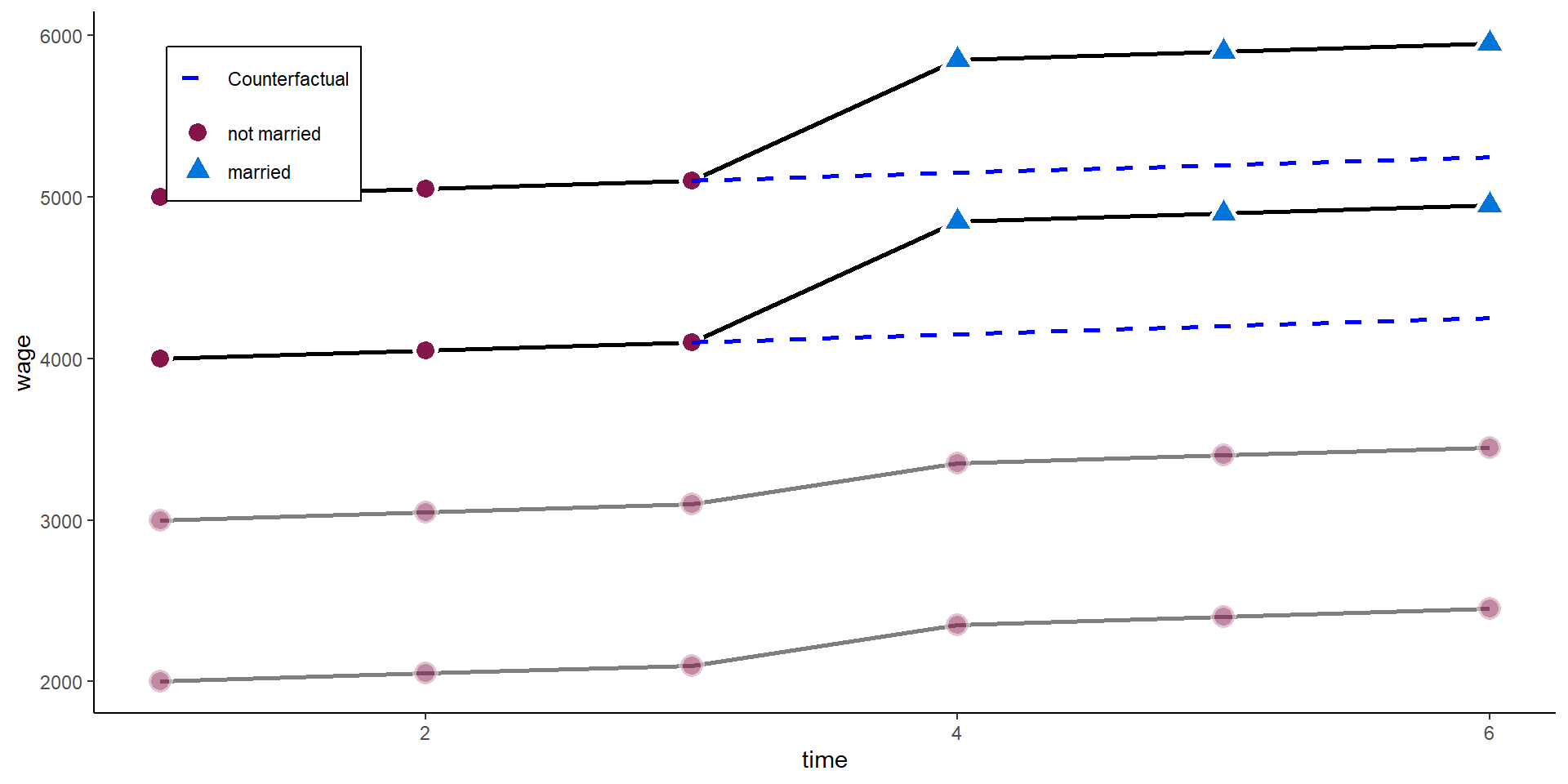
Two-ways FE

To circumvent the problem above, we want to add the never-married as a control group in our estimator.

Tip

In general, it is always a good idea to control for temporal shocks!

Two-ways FE

The two-way FE

\[ y_{it} = \beta x_{it} + \alpha_i + \zeta_t + \epsilon_{it}, \]

adds \(\zeta_t\), with are time fixed effects. Analogous to \(\alpha_i\), we could just add a dummy variable for each year / time period in the data.

This removes common time shocks independent of treatment, and takes back in individuals without variation in \(x\). We basically add a ‘control-group’ to the estimation.

Two-ways FE

In practice, we usually use a transformation approach, where we subtract the between variance by using the person-specific & time-specific means:

\[ \begin{split} (y_{it} - \bar{y}_i - \bar{y}_t + \bar{y}) = \beta (x_{it} - \bar{x}_i - \bar{x}_t + \bar{x}) \\ + (\epsilon_{it} - \bar{\epsilon}_i - \bar{\epsilon}_t + \bar{\epsilon}). \end{split} \]

Two-ways FE

We can just change the effect option in plm to “twoways” to achieve this:

fe3 <- plm(wage ~ marriage, data = df2,
           index = c("id", "time"),
           effect = "twoways", model = "within")
summary(fe3)

Two-ways FE

Or we add another factor variable in `felm’:

fe3_alt <- felm(wage ~ marriage | id + as.factor(time) | 0 | id,
                data = df2)
summary(fe3_alt)

Call:
   felm(formula = wage ~ marriage | id + as.factor(time) | 0 | id,      data = df2) 

Residuals:
       Min         1Q     Median         3Q        Max 
-2.842e-14 -2.842e-14  0.000e+00  2.842e-14  2.842e-14 

Coefficients:
                 Estimate Cluster s.e.  t value Pr(>|t|)    
marriagemarried 5.000e+02    6.711e-14 7.45e+15   <2e-16 ***
---
Signif. codes:  0 '***' 0.001 '**' 0.01 '*' 0.05 '.' 0.1 ' ' 1

Residual standard error: 3.721e-14 on 14 degrees of freedom
Multiple R-squared(full model):     1   Adjusted R-squared:     1 
Multiple R-squared(proj model):     1   Adjusted R-squared:     1 
F-statistic(full model, *iid*):3.125e+33 on 9 and 14 DF, p-value: < 2.2e-16 
F-statistic(proj model): 5.551e+31 on 1 and 3 DF, p-value: < 2.2e-16 

Two-ways FE

Code

### Plot 
zp4 <- ggplot(df2, aes(time, wage)) +
  geom_line(aes(x = time, y = wage, group = id), lty = "solid", colour = "black", lwd = 1) + 
  geom_point( aes(x = time, y = wage, shape = marriage, fill = marriage), 
              size = 4, stroke = 1.5, color = "white") +
  geom_line(aes(x = time, y = pt, group = id, linetype = "dashed"), colour = "blue", lwd = 1) +
  scale_linetype_identity(labels = "Counterfactual", guide = "legend") +
  theme_classic() +
  scale_shape_manual(values = c(21, 24)) +
  scale_fill_manual(values = c("#85144b", "#0074D9")) +
  scale_color_manual(values = c("#85144b", "#0074D9")) +
  theme(legend.key = element_blank(), legend.title = element_blank(),
        legend.position = c(0.05,0.95), legend.justification = c("left", "top"),
        legend.background = element_blank(),
        legend.box.background = element_rect(colour = "black"),
        legend.spacing.y = unit(-0.1, "cm"))
zp4

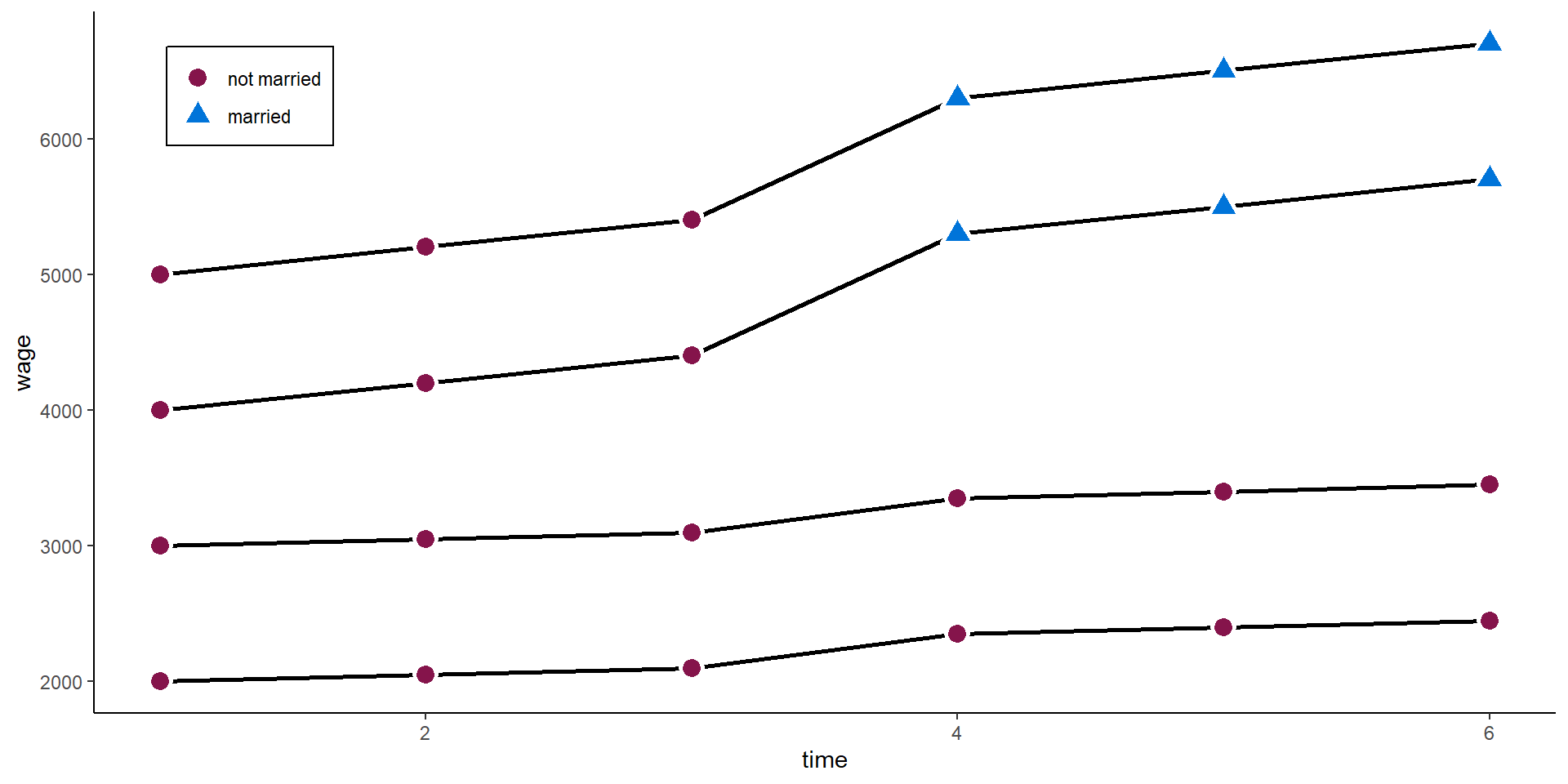
A very critical assumption

In the example above, the twoways FE model works very well. However, adding the control group back in comes with a strong assumption:

Parallel trends between “treatment” and “control” units

Comparing the 3 waves before the treatment above, this assumption here holds. Both - those who marry and those who never marry - have the same time trend in wages before the “treated” marry.

A very critical assumption

Code

zp5 <- ggplot(df2, aes(time, wage2)) +
  geom_line(aes(x = time, y = wage2, group = id), lty = "solid", colour = "black", lwd = 1) + 
  geom_point( aes(x = time, y = wage2, shape = marriage, fill = marriage), 
              size = 4, stroke = 1.5, color = "white") +
  # geom_line(aes(x = time, y = pt2, group = id, linetype = "dashed"), colour = "blue", lwd = 1) +
  # geom_line(aes(x = time, y = pt2_cr, group = id, linetype = "dashed"), colour = "grey", lwd = 1, show.legend = FALSE, alpha = 0.7) +
  scale_linetype_identity(labels = "Counterfactual", guide = "legend") +
  # scale_alpha_manual(values = c(0.3, 1), guide = "none") +
  # ylim(3.3, 9.2) + expand_limits(y = c(0, 0)) + 
  theme_classic() +
  scale_shape_manual(values = c(21, 24)) +
  scale_fill_manual(values = c("#85144b", "#0074D9")) +
  scale_color_manual(values = c("#85144b", "#0074D9")) +
  ylab("wage") +
  theme(legend.key = element_blank(), legend.title = element_blank(),
        legend.position = c(0.05,0.95), legend.justification = c("left", "top"),
        legend.background = element_blank(),
        legend.box.background = element_rect(colour = "black"),
        legend.spacing.y = unit(-0.1, "cm"))
zp5

A very critical assumption

fe3 <- plm(wage2 ~ marriage, data = df2,
           index = c("id", "time"),
           effect = "twoways", model = "within")
summary(fe3)

Twoways effects Within Model

Call:
plm(formula = wage2 ~ marriage, data = df2, effect = "twoways", 
    model = "within", index = c("id", "time"))

Balanced Panel: n = 4, T = 6, N = 24

Residuals:
   Min. 1st Qu.  Median 3rd Qu.    Max. 
    -75     -75       0      75      75 

Coefficients:
                Estimate Std. Error t-value  Pr(>|t|)    
marriagemarried  950.000     65.465  14.511 7.881e-10 ***
---
Signif. codes:  0 '***' 0.001 '**' 0.01 '*' 0.05 '.' 0.1 ' ' 1

Total Sum of Squares:    1443800
Residual Sum of Squares: 90000
R-Squared:      0.93766
Adj. R-Squared: 0.89759
F-statistic: 210.583 on 1 and 14 DF, p-value: 7.8808e-10

Difference in Differences

Difference in Differences

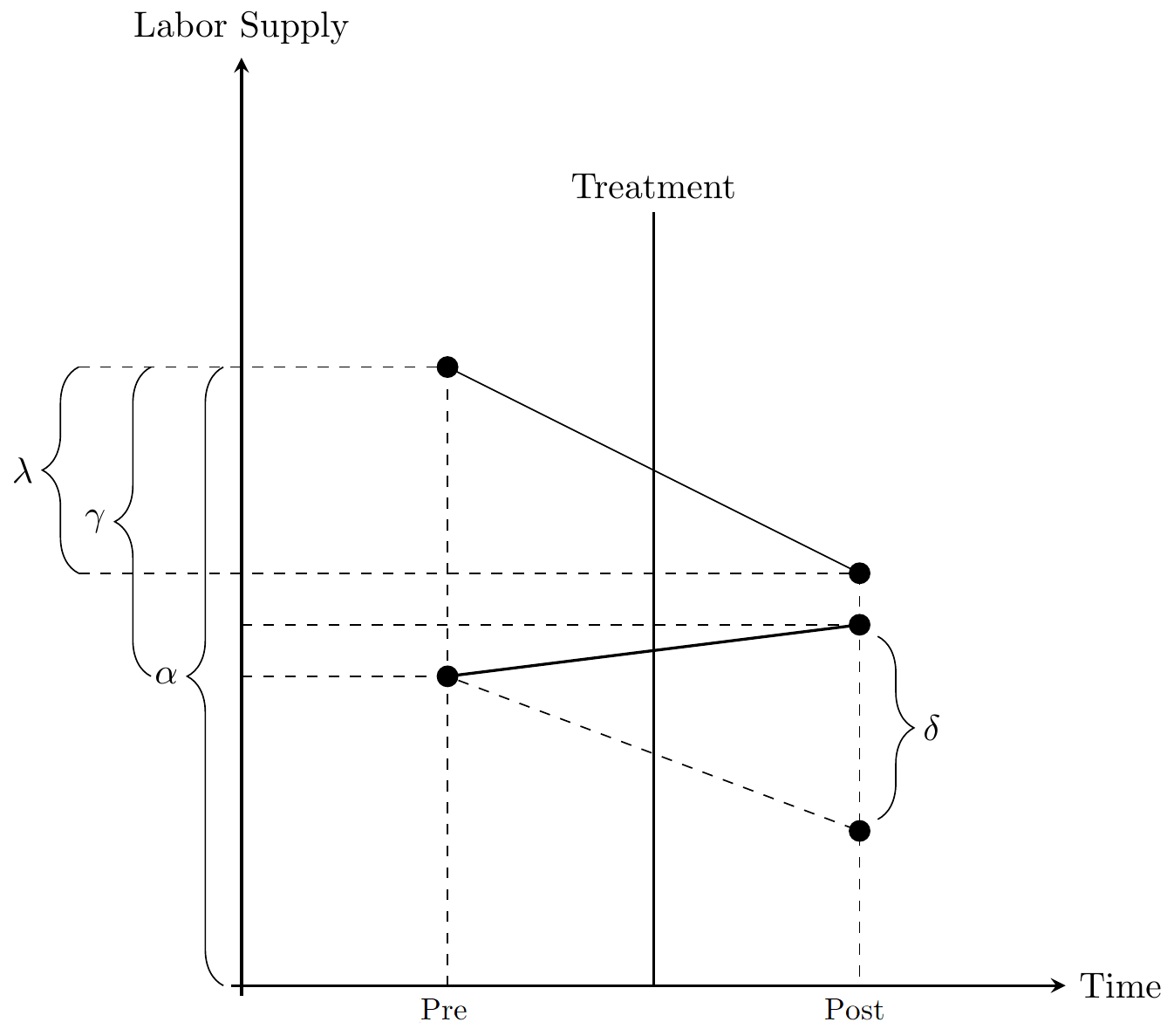
The difference-in-differences (DD) design is a very basic and popular design to identify causal treatment effects in a panel data setting.

The most basic setting, is a \(2\times 2\) DD estimator. It consists of a setting where we have 2 groups: a treatment group (\(T\)) and control group (\(C\)). Each group has been observed at 2 time points: before treatment (\(pre\)) and after treatment (\(post\)).

See Cunningham (2021) and Huntington-Klein (2021).

Difference in Differences

In this setting we can calculate the change in the treatment group: \[ \mathrm{E}(\Delta y_{T}) = \mathrm{E}(y_{T}^{post}) - \mathrm{E}(y_{T}^{pre}), \]

and likewise in the control group: \[ \mathrm{E}(\Delta y_{C}) = \mathrm{E}(y_{C}^{post}) - \mathrm{E}(y_{C}^{pre}). \]

The simple DD estimator is then the difference between the differences in the treatment group and the differences in the control group:

\[ \hat{\delta}_{DD} = \mathrm{E}(\Delta y_{T}) - \mathrm{E}(\Delta y_{C}) = (\mathrm{E}(y_{T}^{post}) - \mathrm{E}(y_{T}^{pre})) - (\mathrm{E}(y_{C}^{post}) - \mathrm{E}(y_{C}^{pre})). \]

Difference in Differences

Diff-in-Diff design, adopted from Cunningham (2021)

Difference in Differences

The DID

\[ y_{it} = \alpha + \gamma D_{i} + \lambda Post_{t} + \delta_{DD} (D_{i} \times Post_{t}) + \upsilon_{it}. \]

is the same estimator in a simple regression, \(D \in {0, 1}\) is a binary indicator of the treatment group and \(Post \in {0, 1}\) a binary indicator of pre- or post-treatment period.

Difference in Differences

The DID

\[ y_{it} = \alpha + \gamma D_{i} + \lambda Post_{t} + \delta_{DD} (D_{i} \times Post_{t}) + \upsilon_{it}. \]

• \(\alpha\): average outcome of control group in pre-treatment period

• \(\gamma\): average difference between treatment and control group in pre-treatment period

• \(\lambda\): average difference between post- pre-treatment period in control group

• \(\delta_{DD}\): difference between treatment and control group in difference between post- pre-treatment period

Difference in Differences

df2$marry_post <- 0
df2$marry_post[df2$time >= 4] <- 1

did1 <- lm(wage ~ marriage_ever*marry_post, data = df2)
summary(did1)

Call:
lm(formula = wage ~ marriage_ever * marry_post, data = df2)

Residuals:
   Min     1Q Median     3Q    Max 
  -550   -500      0    500    550 

Coefficients:
                          Estimate Std. Error t value Pr(>|t|)    
(Intercept)                 2550.0      224.4  11.366 3.53e-10 ***
marriage_ever1              2000.0      317.3   6.304 3.74e-06 ***
marry_post                   350.0      317.3   1.103    0.283    
marriage_ever1:marry_post    500.0      448.7   1.114    0.278    
---
Signif. codes:  0 '***' 0.001 '**' 0.01 '*' 0.05 '.' 0.1 ' ' 1

Residual standard error: 549.5 on 20 degrees of freedom
Multiple R-squared:  0.8449,    Adjusted R-squared:  0.8217 
F-statistic: 36.32 on 3 and 20 DF,  p-value: 2.757e-08

Difference in Differences

In a setting where \(T=2\) or in a setting where every observation is treated at the same time, the DD equals the two-ways FE.

In general, DD and two-ways DD are often seen as equivalents. However, the situation becomes more complicated when treatment timing varies (Goodman-Bacon 2021).

Tip

When estimating FE or Diff-in-Diff estimators, “one should restrict the estimation sample to those persons who can potentially experience the treatment during the observation window”. Usually this means that we start with the not-yet-treated and omit the already-treated (Brüderl and Ludwig 2015).

Random Effects

Random effects estimator

The RE estimator

\[ y_{it} = \alpha + \beta x_{it} + \alpha_i + \vartheta_{it}. \]

Instead of assuming \(\alpha_i\) are fixed effects, we treat them as i.i.d random effects, usually assuming they are normally distributed

Random effects estimator

The RE estimator has two main “advantages” over the FE estimator:

1. It is more efficient if \(\mathrm{E}(\alpha_{i} | x_{it}) = 0\): it has lower standard errors

2. It allows to estimate the effects of time-constant variables

Random effects estimator

However, it obscures the main advantage of panel data: the relaxation of assumptions for consistency of estimators. The RE estimator needs the same assumptions as POLS for consistency:

• \(\mathrm{E}(\alpha_{i} | x_{it}) = 0\): No time-constant unobserved heterogeneity

• \(\mathrm{E}(\epsilon_{it} | x_{it}) = 0\): No time-varying unobserved heterogeneity

Random effects estimator

We can also write the RE as a quasi-demeaned estimator:

\[ (y_{it} - \lambda\bar{y}_i) = \beta (x_{it} - \lambda\bar{x}_i) + (\epsilon_{it} - \lambda\bar{\epsilon}_i) \]

where \(\hat{\lambda} = 1 - \sqrt{\frac{\sigma^2_\epsilon}{\sigma^2_\epsilon + T\sigma^2_\alpha}}\), with \(\sigma^2_\epsilon\) denoting the residual variance, and \(\sigma^2_\alpha\) denoting the variance of the individual effects \(\alpha_i\).

Random effects estimator

The RE (as POLS) is thus a weighted average of between and within estimator. The weights are determined by the residual variance in FE as share of total residual variance:

\[ \begin{split} \beta_{RE} = \omega_{GLS} \beta_{FE} + (1-\omega_{GLS}) \beta_{BE},\\ \omega_{GLS} = \frac{\sigma^2_{\tilde{x}}}{\sigma^2_{\tilde{x}} + \phi^2 (\sigma^2_x-\sigma^2_{\tilde{x}})},\\ \phi = \sqrt{\frac{\hat{\sigma}^2_{FE}}{\hat{\sigma}^2_{BE}}}, \end{split} \]

Random effects estimator

It thus follows that:

• \(T\) large, \(\sigma^2_\alpha\) large, then RE \(\rightarrow\) FE

• \(\sigma^2_\alpha\) small, then RE \(\rightarrow\) POLS

The RE uses all the available information - between and within variance - and weights the two components by its “predictive power”. This makes it the most efficient estimator.

RE in plm

Let’s estimate the RE for the happiness - age example, again using the plm package.

Code

re1 <- plm(happiness ~ age, data = df,
           index = c("id", "time"),
           effect = "individual", model = "random")
summary(re1)

RE in plm

Let’s estimate the RE for the happiness - age example, again using the plm package.

Code

re1 <- plm(happiness ~ age, data = df,
           index = c("id", "time"),
           effect = "individual", model = "random")
summary(re1)

Oneway (individual) effect Random Effect Model 
   (Swamy-Arora's transformation)

Call:
plm(formula = happiness ~ age, data = df, effect = "individual", 
    model = "random", index = c("id", "time"))

Balanced Panel: n = 6, T = 4, N = 24

Effects:
                  var std.dev share
idiosyncratic 0.03641 0.19081 0.096
individual    0.34396 0.58648 0.904
theta: 0.8394

Residuals:
     Min.   1st Qu.    Median   3rd Qu.      Max. 
-1.054061 -0.353296  0.013426  0.316500  0.898703 

Coefficients:
             Estimate Std. Error z-value  Pr(>|z|)    
(Intercept)  6.933947   1.534054  4.5200 6.183e-06 ***
age         -0.015621   0.031277 -0.4994    0.6175    
---
Signif. codes:  0 '***' 0.001 '**' 0.01 '*' 0.05 '.' 0.1 ' ' 1

Total Sum of Squares:    5.1257
Residual Sum of Squares: 5.0683
R-Squared:      0.011211
Adj. R-Squared: -0.033734
Chisq: 0.249442 on 1 DF, p-value: 0.61747

Equal weights of within and between

Code

N <- 6
T <- 4
### Models
# Total line for plot
lm1 <- lm(happiness ~ age, data = df)
lm2 <- lm(happiness ~ age + cohort, data = df)
lm3 <- lm(happiness ~ age + idname, data = df)
lm4 <- lm(m_happiness ~ m_age, data = df)
re <- plm(happiness ~ age, df, model = "random", effect = "individual")

### Compare POLS, BE, FE, and RE
estimates <- data.frame(matrix(NA, ncol = 3, nrow = 4))
names(estimates) <- c("Model", "Intercept", "slope")
estimates[1,] <- c("POLS",
                   lm1$coefficients[1],
                   lm1$coefficients[2])
estimates[2,] <- c("BE",
                   lm4$coefficients[1], 
                   lm4$coefficients[2])
estimates[3,] <- c("FE",
                   lm3$coefficients[1] + 1/N * lm3$coefficients[3]  + 1/N * lm3$coefficients[4] 
                   + 1/N * lm3$coefficients[5]  + 1/N * lm3$coefficients[6]  + 1/N * lm3$coefficients[7], 
                   lm3$coefficients[2])
estimates[4,] <- c("RE",
                   re$coefficients[1], 
                   re$coefficients[2])
estimates[, -1] <- apply(estimates[, -1], 2, FUN = function(x) as.numeric(x))

newdf <- data.frame(matrix(NA, ncol = 2, nrow = 2))
names(newdf) <- c("x", "y")
newdf$x <- c(min(df$age), max(df$age))
for(i in 1:nrow(estimates)){
  newdf$y <- estimates[i, "Intercept"] + estimates[i, "slope"]*newdf$x
  newdf$Model <- estimates[i, "Model"]
  if(i == 1){
    pred <- newdf
  }else{pred <- rbind(pred, newdf)}
}

estimates$Model <- factor(estimates$Model, levels = c("POLS", "BE", "FE", "RE"))

gg_color_hue <- function(n) {
  hues = seq(15, 375, length = n + 1)
  hcl(h = hues, l = 65, c = 100)[1:n]
}

zp6 <- ggplot(df, aes(age, happiness)) +
  geom_point(aes(x = age, y = happiness, shape = idname),
             colour = rep(gg_color_hue(6), each = T),
              size = 2, stroke = 1, show.legend = FALSE) +
  geom_smooth(method = 'lm', formula = y ~ x, se = FALSE, show.legend = FALSE,
              linetype = "dashed", aes(group = idname), colour = alpha("gray", 1)) +
  geom_point(data = unique(df[, c("m_age", "m_happiness", "idname")]),
             aes(x = m_age, y = m_happiness, shape = idname),
             colour = gg_color_hue(6), alpha = 0.5,
              size = 3, stroke = 2, show.legend = FALSE) +
  scale_fill_manual(values = cbp2[-c(1, 2)]) +
  scale_colour_manual(values = cbp2[-c(1, 2)]) + 
  scale_shape_manual(values = c(15:18, 25, 20)) +
  geom_abline(data = estimates, lwd = 1.2,
              mapping = aes(intercept = Intercept, slope = slope, 
                            colour = Model, linetype = Model)) +
  scale_linetype_manual(values = c("solid", "twodash", "longdash", "dotdash")) +
  scale_color_viridis(discrete = TRUE, option = "D")+
  ylim(3.3, 9.2) + expand_limits(y = c(0, 0)) + 
  theme_classic() +
  theme(legend.key = element_blank(), legend.title = element_blank(),
        legend.position = c(0.95,0.05), legend.justification = c("right", "bottom"),
        legend.background = element_blank(),
        legend.box.background = element_rect(colour = "black"),
        plot.title = element_text(hjust = 0.5))
zp6

Increasing T

Code

N <- 6
T <- 8

set.seed(123)
df <- simdata(N = N, T = T, uw_sd = 0, age_range = c(20:60))

### Models
# Total line for plot
lm1 <- lm(happiness ~ age, data = df)
lm2 <- lm(happiness ~ age + cohort, data = df)
lm3 <- lm(happiness ~ age + idname, data = df)
lm4 <- lm(m_happiness ~ m_age, data = df)
re <- plm(happiness ~ age, df, model = "random", effect = "individual")

### Compare POLS, BE, FE, and RE
estimates <- data.frame(matrix(NA, ncol = 3, nrow = 4))
names(estimates) <- c("Model", "Intercept", "slope")
estimates[1,] <- c("POLS",
                   lm1$coefficients[1],
                   lm1$coefficients[2])
estimates[2,] <- c("BE",
                   lm4$coefficients[1], 
                   lm4$coefficients[2])
estimates[3,] <- c("FE",
                   lm3$coefficients[1] + 1/N * lm3$coefficients[3]  + 1/N * lm3$coefficients[4] 
                   + 1/N * lm3$coefficients[5]  + 1/N * lm3$coefficients[6]  + 1/N * lm3$coefficients[7], 
                   lm3$coefficients[2])
estimates[4,] <- c("RE",
                   re$coefficients[1], 
                   re$coefficients[2])
estimates[, -1] <- apply(estimates[, -1], 2, FUN = function(x) as.numeric(x))

newdf <- data.frame(matrix(NA, ncol = 2, nrow = 2))
names(newdf) <- c("x", "y")
newdf$x <- c(min(df$age), max(df$age))
for(i in 1:nrow(estimates)){
  newdf$y <- estimates[i, "Intercept"] + estimates[i, "slope"]*newdf$x
  newdf$Model <- estimates[i, "Model"]
  if(i == 1){
    pred <- newdf
  }else{pred <- rbind(pred, newdf)}
}

estimates$Model <- factor(estimates$Model, levels = c("POLS", "BE", "FE", "RE"))

gg_color_hue <- function(n) {
  hues = seq(15, 375, length = n + 1)
  hcl(h = hues, l = 65, c = 100)[1:n]
}

zp7 <- ggplot(df, aes(age, happiness)) +
  geom_point(aes(x = age, y = happiness, shape = idname),
             colour = rep(gg_color_hue(6), each = T),
              size = 2, stroke = 1, show.legend = FALSE) +
  geom_smooth(method = 'lm', formula = y ~ x, se = FALSE, show.legend = FALSE,
              linetype = "dashed", aes(group = idname), colour = alpha("gray", 1)) +
  geom_point(data = unique(df[, c("m_age", "m_happiness", "idname")]),
             aes(x = m_age, y = m_happiness, shape = idname),
             colour = gg_color_hue(6), alpha = 0.5,
              size = 3, stroke = 2, show.legend = FALSE) +
  scale_fill_manual(values = cbp2[-c(1, 2)]) +
  scale_colour_manual(values = cbp2[-c(1, 2)]) + 
  scale_shape_manual(values = c(15:18, 25, 20)) +
  geom_abline(data = estimates, lwd = 1.2,
              mapping = aes(intercept = Intercept, slope = slope, 
                            colour = Model, linetype = Model)) +
  scale_linetype_manual(values = c("solid", "twodash", "longdash", "dotdash")) +
  scale_color_viridis(discrete = TRUE, option = "D")+
  scale_linetype_manual(values = c("solid", "twodash", "longdash", "dotdash")) +
  ylim(3.3, 9.2) + expand_limits(y = c(0, 0)) + 
  theme_classic() +
  theme(legend.key = element_blank(), legend.title = element_blank(),
        legend.position = c(0.95,0.05), legend.justification = c("right", "bottom"),
        legend.background = element_blank(),
        legend.box.background = element_rect(colour = "black"),
        plot.title = element_text(hjust = 0.5))
zp7

Increasing the within-unit noise

Code

N <- 6
T <- 8

set.seed(123)
df <- simdata(N = N, T = T, uw_sd = 0.5, age_range = c(20:60))

### Models
# Total line for plot
lm1 <- lm(happiness ~ age, data = df)
lm2 <- lm(happiness ~ age + cohort, data = df)
lm3 <- lm(happiness ~ age + idname, data = df)
lm4 <- lm(m_happiness ~ m_age, data = df)
re <- plm(happiness ~ age, df, model = "random", effect = "individual")

### Compare POLS, BE, FE, and RE
estimates <- data.frame(matrix(NA, ncol = 3, nrow = 4))
names(estimates) <- c("Model", "Intercept", "slope")
estimates[1,] <- c("POLS",
                   lm1$coefficients[1],
                   lm1$coefficients[2])
estimates[2,] <- c("BE",
                   lm4$coefficients[1], 
                   lm4$coefficients[2])
estimates[3,] <- c("FE",
                   lm3$coefficients[1] + 1/N * lm3$coefficients[3]  + 1/N * lm3$coefficients[4] 
                   + 1/N * lm3$coefficients[5]  + 1/N * lm3$coefficients[6]  + 1/N * lm3$coefficients[7], 
                   lm3$coefficients[2])
estimates[4,] <- c("RE",
                   re$coefficients[1], 
                   re$coefficients[2])
estimates[, -1] <- apply(estimates[, -1], 2, FUN = function(x) as.numeric(x))

newdf <- data.frame(matrix(NA, ncol = 2, nrow = 2))
names(newdf) <- c("x", "y")
newdf$x <- c(min(df$age), max(df$age))
for(i in 1:nrow(estimates)){
  newdf$y <- estimates[i, "Intercept"] + estimates[i, "slope"]*newdf$x
  newdf$Model <- estimates[i, "Model"]
  if(i == 1){
    pred <- newdf
  }else{pred <- rbind(pred, newdf)}
}

estimates$Model <- factor(estimates$Model, levels = c("POLS", "BE", "FE", "RE"))

gg_color_hue <- function(n) {
  hues = seq(15, 375, length = n + 1)
  hcl(h = hues, l = 65, c = 100)[1:n]
}

zp7 <- ggplot(df, aes(age, happiness)) +
  geom_point(aes(x = age, y = happiness, shape = idname),
             colour = rep(gg_color_hue(6), each = T),
              size = 2, stroke = 1, show.legend = FALSE) +
  geom_smooth(method = 'lm', formula = y ~ x, se = FALSE, show.legend = FALSE,
              linetype = "dashed", aes(group = idname), colour = alpha("gray", 1)) +
  geom_point(data = unique(df[, c("m_age", "m_happiness", "idname")]),
             aes(x = m_age, y = m_happiness, shape = idname),
             colour = gg_color_hue(6), alpha = 0.5,
              size = 3, stroke = 2, show.legend = FALSE) +
  scale_fill_manual(values = cbp2[-c(1, 2)]) +
  scale_colour_manual(values = cbp2[-c(1, 2)]) + 
  scale_shape_manual(values = c(15:18, 25, 20)) +
  geom_abline(data = estimates, lwd = 1.2,
              mapping = aes(intercept = Intercept, slope = slope, 
                            colour = Model, linetype = Model)) +
  scale_linetype_manual(values = c("solid", "twodash", "longdash", "dotdash")) +
  scale_color_viridis(discrete = TRUE, option = "D")+
  ylim(3.3, 9.2) + expand_limits(y = c(0, 0)) + 
  theme_classic() +
  theme(legend.key = element_blank(), legend.title = element_blank(),
        legend.position = c(0.95,0.05), legend.justification = c("right", "bottom"),
        legend.background = element_blank(),
        legend.box.background = element_rect(colour = "black"),
        plot.title = element_text(hjust = 0.5))
zp7

References

Brüderl, Josef, and Volker Ludwig. 2015. “Fixed-Effects Panel Regression.” In The Sage Handbook of Regression Analysis and Causal Inference, edited by Henning Best and Christof Wolf, 327–57. Los Angeles: Sage.

Cunningham, Scott. 2021. Causal Inference: The Mixtape. New Haven and London: Yale University Press.

Goodman-Bacon, Andrew. 2021. “Difference-in-Differences with Variation in Treatment Timing.” Journal of Econometrics 225 (2): 254–77. https://doi.org/10.1016/j.jeconom.2021.03.014.

Huntington-Klein, Nick. 2021. The Effect: An Introduction to Research Design and Causality. Boca Raton: Chapman & Hall/CRC.

Wooldridge, Jeffrey M. 2010. Econometric Analysis of Cross Section and Panel Data. Cambridge, Mass.: MIT Press.